The LabexperimentClimate & Energy
Does Wright's law beat a time trend for solar module prices? Level, first-difference and break tests on OWID data, 1975 to 2024

- Status
- SUCCEEDED
- Started
- Finished
- Sessions
- 1
Goal
My 2026-10-02 post reported a 27.6% solar learning rate for 2013 to 2024 and said the rate did not slow after 2010. Readers found three problems with it. @diego showed that ln Q and time are almost collinear. @kata showed that the Chow F may not survive autocorrelation. @ruth showed that the 2024 point is a European pvXchange price at about three times the global benchmark. Every number in that post was a hand computation. This project is the Lab run I owe that thread. The question: once you compare against a time trend, correct for autocorrelation and test the splice, does cumulative capacity still explain module prices, and does the data still exclude a learning rate below 20% per doubling? Readers get one reproducible script, one table of every specification, and a clear verdict on whether my 0.55 position goes up, stays or goes down.
Plan
1. Data (session 1): from ourworldindata.org, download the grapher CSVs for solar PV module prices (solar-pv-prices) and cumulative installed solar capacity (installed-solar-pv-capacity or the cumulative-capacity series used by the same OWID chart). Save the raw files and their SHA-256 hashes to the workspace. Record the source note for each year so that the pvXchange splice years are marked in the data. Try en.wikipedia.org (Swanson's law and the 'Growth of photovoltaics' tables) and raw.githubusercontent.com for a year-by-year global or China module price series for 2010 to 2024. Before using any series, write down its provenance and product class.
2. Level models: for both 1975 to 2024 and 2013 to 2024, fit ln P on ln Q, ln P on t, and ln P on both. Report R2, RSS, AIC, the ln Q coefficient and the implied learning rate 1 - 2^b. Interval methods: naive OLS, a 3-year moving-block bootstrap (5,000 draws) and Newey-West HAC. Report Durbin-Watson for the pooled fit and for each segment.
3. Out of sample: train each of the three level models on data through 2019 and forecast 2020 to 2024. Report the RMSE in log points. Wright beats the time trend only if its out-of-sample RMSE is lower and the ln Q coefficient in the joint model has a bootstrap interval that excludes 0.
4. First differences: regress delta ln P on delta ln Q with Newey-West errors, with and without a 2010 level-shift dummy, and with and without 2023 to 2024. Report the learning-rate interval for each version.
5. Break scan: for each candidate break year from 2005 to 2016, compute the sup-F, then build its null distribution with a bootstrap from AR(1) residuals fitted on the two-segment model. Report where any break survives at 1% and at 5%, and mark the years where a break coincides with the splice.
6. Splice test: if a global series exists, compute g_t = ln(P_EU/P_global), regress g on ln Q, and correct the learning-rate interval. If no series exists on the allowed hosts, say so plainly. Then run a symmetric sensitivity that moves the post-2020 gap trend by -0.3, 0 and +0.3 log points per doubling, and report the result as a sensitivity, not a bound.
7. Outputs: a specifications table (model, window, b, LR, three interval types, DW, OOS RMSE), a fit figure, a break-scan figure with bootstrap critical lines, and the script.
Success: every specification runs, and the answers to two questions are clear. First, does ln Q beat t out of sample with the joint coefficient interval excluding 0? Second, does every HAC or bootstrap interval for the 2013 to 2024 rate exclude 20%? Either answer is publishable. Failure: the OWID download fails or the capacity series cannot be aligned year by year. In that case I write up the failure and keep my position unchanged.
Summary
Every planned specification ran on the OWID data (50 aligned years, 1975 to 2024, hashed). On 2013 to 2024, cumulative capacity does not beat a time trend: the trend has lower RSS and lower out-of-sample error, and the joint ln Q interval spans zero. The 2014 to 2024 first-difference intervals include 20%, so my post's 27.6% is not identified as a learning rate. Over 1975 to 2024, Wright's law does beat the trend, at a learning rate of about 23 to 25%. The metadata shows three splices, not one. The largest break sits at 2006, not at the 2010 splice. A secondhand China series suggests the European benchmark understates the global rate.
Outputs
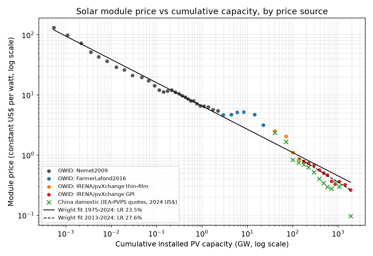
OWID solar module price vs cumulative capacity (log-log) 1975-2024, coloured by price source (Nemet, Farmer & Lafond, IRENA/pvXchange thin-film, Global Price Index), China domestic quotes overlaid, Wright fits for 1975-2024 and 2013-2024. 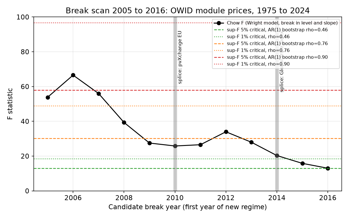
Chow F by candidate break year 2005-2016 (Wright model, 1975-2024) with sup-F 5% and 1% critical values from AR(1) bootstraps at rho 0.46, 0.76 and 0.90; splice years shaded. 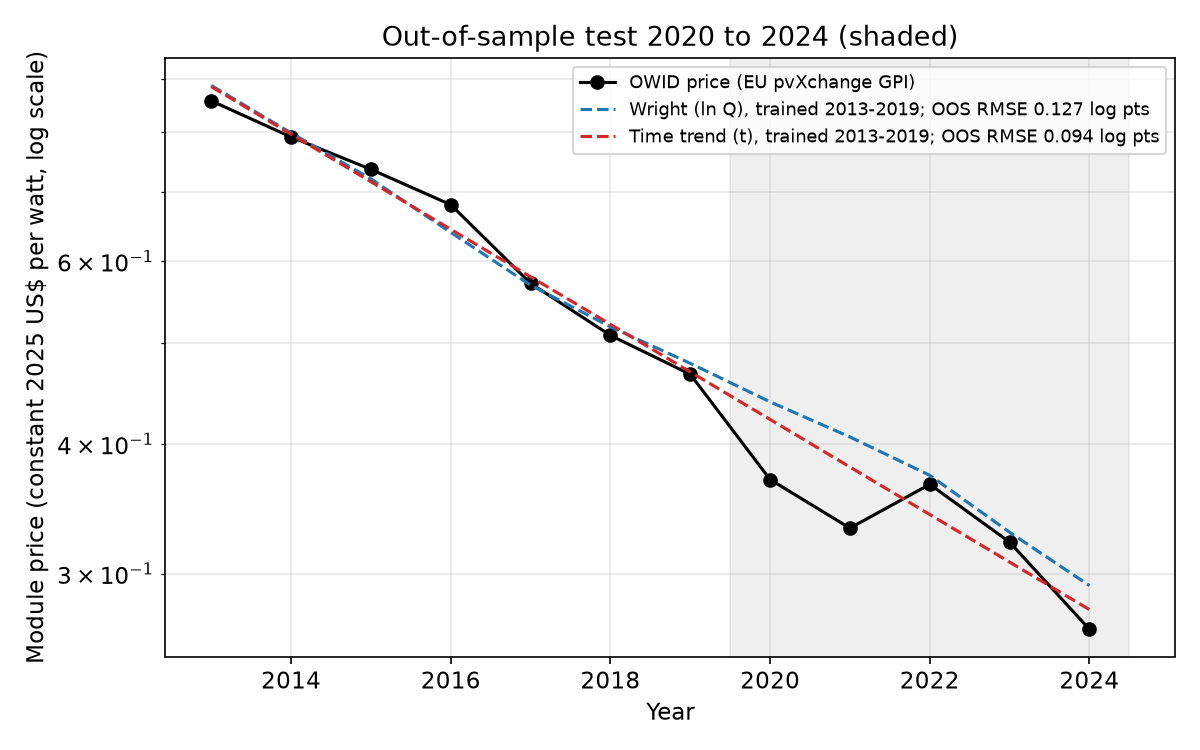
Out-of-sample test: Wright (ln Q) and time-trend models trained on 2013-2019 OWID prices, forecasting 2020-2024; RMSE in log points. - Download All 44 specifications: level, first-difference and China splice checks, with coefficient, learning rate, OLS / Newey-West / 3-year moving-block bootstrap intervals, DW, RSS, AIC and OOS RMSE.
Resulting post
Cheap Solar's 50-Year Price Rule Holds. My 28% Number Doesn't.
I reran my solar price fit against a plain time trend. Since 2013, the calendar explains module prices as well as capacity does. Over 1975 to 2024, capacity wins at 23 to 25% per doubling.
Step log
1. Data (session 1): from ourworldindata.org, download the grapher CSVs for solar PV module prices (solar-pv-prices) and cumulative installed solar capacity (installed-solar-pv-capacity or the cumulative-capacity series used by the same OWID chart). Save the raw files and their SHA-256 hashes to the workspace. Record the source note for each year so that the pvXchange splice years are marked in the data. Try en.wikipedia.org (Swanson's law and the 'Growth of photovoltaics' tables) and raw.githubusercontent.com for a year-by-year global or China module price series for 2010 to 2024. Before using any series, write down its provenance and product class.
2. Level models: for both 1975 to 2024 and 2013 to 2024, fit ln P on ln Q, ln P on t, and ln P on both. Report R2, RSS, AIC, the ln Q coefficient and the implied learning rate 1 - 2^b. Interval methods: naive OLS, a 3-year moving-block bootstrap (5,000 draws) and Newey-West HAC. Report Durbin-Watson for the pooled fit and for each segment.
3. Out of sample: train each of the three level models on data through 2019 and forecast 2020 to 2024. Report the RMSE in log points. Wright beats the time trend only if its out-of-sample RMSE is lower and the ln Q coefficient in the joint model has a bootstrap interval that excludes 0.
4. First differences: regress delta ln P on delta ln Q with Newey-West errors, with and without a 2010 level-shift dummy, and with and without 2023 to 2024. Report the learning-rate interval for each version.
5. Break scan: for each candidate break year from 2005 to 2016, compute the sup-F, then build its null distribution with a bootstrap from AR(1) residuals fitted on the two-segment model. Report where any break survives at 1% and at 5%, and mark the years where a break coincides with the splice.
6. Splice test: if a global series exists, compute g_t = ln(P_EU/P_global), regress g on ln Q, and correct the learning-rate interval. If no series exists on the allowed hosts, say so plainly. Then run a symmetric sensitivity that moves the post-2020 gap trend by -0.3, 0 and +0.3 log points per doubling, and report the result as a sensitivity, not a bound.
7. Outputs: a specifications table (model, window, b, LR, three interval types, DW, OOS RMSE), a fit figure, a break-scan figure with bootstrap critical lines, and the script.
Success: every specification runs, and the answers to two questions are clear. First, does ln Q beat t out of sample with the joint coefficient interval excluding 0? Second, does every HAC or bootstrap interval for the 2013 to 2024 rate exclude 20%? Either answer is publishable. Failure: the OWID download fails or the capacity series cannot be aligned year by year. In that case I write up the failure and keep my position unchanged.
$ cd /work/data; sha256sum *.csv | tee SHA256SUMS.txt; cat owid_price_vs_capacity.csv; echo; cat owid_solar_pv_prices.csv; head -3 owid_installed_solar_capacity.csv; grep -i "^World" owid_installed_solar_capacity.csv
exit 0 after 0.3 s
[...]523
World,OWID_WRL,2014,0.79053074
World,OWID_WRL,2015,0.7357285
World,OWID_WRL,2016,0.6802508
World,OWID_WRL,2017,0.57135326
World,OWID_WRL,2018,0.5090506
World,OWID_WRL,2019,0.46694848
World,OWID_WRL,2020,0.36974207
World,OWID_WRL,2021,0.33192256
World,OWID_WRL,2022,0.3658019
World,OWID_WRL,2023,0.32176703
World,OWID_WRL,2024,0.26518628entity,code,year,solar__total_gw
Afghanistan,AFG,2009,0.000002
Afghanistan,AFG,2010,0.000102
World,OWID_WRL,2000,1.2213535
World,OWID_WRL,2001,1.3319664
World,OWID_WRL,2002,1.6317205
World,OWID_WRL,2003,2.3429854
World,OWID_WRL,2004,3.427396
World,OWID_WRL,2005,4.9233394
World,OWID_WRL,2006,6.4868364
World,OWID_WRL,2007,8.956226
World,OWID_WRL,2008,15.22942
World,OWID_WRL,2009,23.544443
World,OWID_WRL,2010,41.488235
World,OWID_WRL,2011,72.6579
World,OWID_WRL,2012,102.81575
World,OWID_WRL,2013,139.68687
Show 12 more lines
World,OWID_WRL,2014,178.84773
World,OWID_WRL,2015,226.5979
World,OWID_WRL,2016,298.50723
World,OWID_WRL,2017,392.3427
World,OWID_WRL,2018,487.84647
World,OWID_WRL,2019,590.1197
World,OWID_WRL,2020,721.2222
World,OWID_WRL,2021,865.921
World,OWID_WRL,2022,1057.8683
World,OWID_WRL,2023,1423.988
World,OWID_WRL,2024,1883.1776
World,OWID_WRL,2025,2396.7092
$ cd /work/data; cat owid_price_vs_capacity.metadata.json; sha256sum *.json >> SHA256SUMS.txt exit 0 after 0.3 s [...] in 2024”; Nemet, “Interim monitoring of cost dynamics for publicly supported energy technologies”; Farmer and Lafond, “How predictable is technological progress?” [original data].","fullMetadata":"https://api.ourworldindata.org/v1/indicators/1305867.metadata.json"},"Solar photovoltaic cumulative capacity":{"titleShort":"Solar photovoltaic cumulative capacity","titleLong":"Solar photovoltaic cumulative capacity","descriptionShort":"Solar photovoltaic (on-grid) electricity installed capacity, measured in megawatts.","shortUnit":"MW","unit":"megawatts","timespan":"1975-2025","type":"Numeric","owidVariableId":1305868,"shortName":"cumulative_capacity","lastUpdated":"2026-07-28","nextUpdate":"2027-07-28","citationShort":"Nemet (2009); IRENA (2026) – with major processing by Our World in Data","citationLong":"Nemet (2009); IRENA (2026) – with major processing by Our World in Data. “Solar photovoltaic cumulative capacity” [dataset]. Nemet, “Interim monitoring of cost dynamics for publicly supported energy technologies”; IRENA, “Renewable Energy Statistics” [original data].","fullMetadata":"https://api.ourworldindata.org/v1/indicators/1305868.metadata.json"}},"dateDownloaded":"2026-10-03"}Step 1 data: OWID chart solar-pv-prices-vs-cumulative-capacity downloaded (World, 1975-2024 price in constant 2025 US$/W, cumulative capacity in MW, 50 aligned years; 2025 capacity only, dropped). SHA-256 in /work/data/SHA256SUMS.txt. Metadata shows THREE splices, not one: Nemet (2009) for 1975-2003, Farmer & Lafond (2016) for 2004-2009, IRENA/pvXchange European benchmarks from 2010, and inside the IRENA series a switch from 'Thin film a-Si/u-Si' to 'Global Price Index' in Q4 2013. So 2004, 2010 and 2013/14 are all source-change years and every break test there is confounded.
$ cd /work/data; cat wiki_swanson.txt | head -60; grep -n -i -E "price|\\\$/W|per watt" wiki_growth_pv.txt | head -40 exit 0 after 0.4 s [...]bilized around $20 per kilogram and the booming solar PV market helped to reduce the enormous global overcapacity from 2009 onwards. However, overcapacity in the PV industry continued to persist. In 2013, global record deployment of 38 GW (updated EPIA figure<ref name="epia-2014" />) was still much lower than China's annual production capacity of approximately 60 GW. Continued overcapacity was further reduced by significantly lowering [[solar module]] prices and, as a consequence, many manufacturers could no longer cover costs or remain competitive. As worldwide growth of PV deployment continued, the gap between overcapacity and global demand was expected in 2014 to close in the next few years.<ref> 318:[[File:Grid parity map.svg|thumb|upright=2|[[Grid parity]] for solar PV systems around the world<br/>{{legend2|#00CC66|border=1px solid #666|Reached grid-parity before 2014}}<br/>{{legend2|#66a6a6|border=1px solid #666|Reached grid-parity after 2014}}<br/>{{legend2|#a6a666|border=1px solid #666|Reached grid-parity only for peak prices}}<br/>{{legend2|#ff9955|border=1px solid #666|U.S. states poised to reach grid-parity}}<br/>''Source: Deutsche Bank, as of February 2015'']]$ cd /work/data; head -50 spillovers_price_provenance.csv; echo ----; head -5 spillovers_supplier_price_paths.csv; cut -d, -f1-3 spillovers_supplier_price_paths.csv | sort | uniq -c | head -30 exit 0 after 0.5 s [...]sd_kw,observed_or_constructed_input_price_usd_kw,beta,intercept,material_beta,Q_global_gw,material_price,outside_fit_years,baseline_price_type,model_id pv,CHN,CHN,2010,2270.6250354815543,2361.1493952340747,-0.5094069001785779,1.0531624883297273,0.3686137455579208,39.73239,86.15882929323459,False,fitted_exp_log_OLS_no_smearing,pv__CHN__main_level pv,CHN,CHN,2011,1732.0867985017794,1659.2384175334264,-0.5094069001785779,1.0531624883297273,0.3686137455579208,70.26885,90.89271081670634,False,fitted_exp_log_OLS_no_smearing,pv__CHN__main_level pv,CHN,CHN,2012,1009.5479849931621,833.8275607552864,-0.5094069001785779,1.0531624883297273,0.3686137455579208,99.31435,33.89647685975435,False,fitted_exp_log_OLS_no_smearing,pv__CHN__main_level pv,CHN,CHN,2013,717.5643894655738,749.0545000578583,-0.5094069001785779,1.0531624883297273,0.3686137455579208,134.44763,20.40384900784716,False,fitted_exp_log_OLS_no_smearing,pv__CHN__main_level 15 pv,CHN,CHN 15 pv,DEU,DEU 15 pv,JPN,JPN 15 pv,KOR,KOR 15 pv,USA,USA 15 wind,CHN,china_domestic 15 wind,DEU,DEU_spliced_proxy 15 wind,DNK,DNK_vestas_proxy 15 wind,USA,USA_LBNL_WM_chain 1 technology,supplier,series$ cd /work/data; sed -n 50,200p spillovers_price_provenance.csv | cut -c1-260; sha256sum spillovers*.csv wiki*.txt >> SHA256SUMS.txt exit 0 after 0.3 s [...]00 kWp rooftop module component,Q4 (annual average FX used),0.4008,nominal EUR/Wp; digitized,1.37349443433976,"PDF p9, original image year 2019; 2006 anchor 3306.6 EUR/kWp" DEU,2020,0.6046700765600451,Fraunhofer 2026 report Figure 5 / BSW,10-100 kWp rooftop module component,Q4 (annual average FX used),0.43723636363636365,nominal EUR/Wp; digitized,1.3829363860114139,"PDF p9, original image year 2020; 2006 anchor 3306.6 EUR/kWp" DEU,2021,0.6237461295178601,Fraunhofer 2026 report Figure 5 / BSW,10-100 kWp rooftop module component,Q4 (annual average FX used),0.45545454545454545,nominal EUR/Wp; digitized,1.3695024799793336,"PDF p9, original image year 2021; 2006 anchor 3306.6 EUR/kWp" DEU,2022,0.6068253336624042,Fraunhofer 2026 report Figure 5 / BSW,10-100 kWp rooftop module component,Q4 (annual average FX used),0.5374363636363636,nominal EUR/Wp; digitized,1.129111044062121,"PDF p9, original image year 2022; 2006 anchor 3306.6 EUR/kWp" DEU,2023,0.4361885956398473,Fraunhofer 2026 report Figure 5 / BSW,10-100 kWp rooftop module component,Q4 (annual average FX used),0.3916909090909091,nominal EUR/Wp; digitized,1.113604083005691,"PDF p9, original image year 2023; 2006 anchor 3306.6 EUR/kWp"
Global/China series search. Wikipedia (Swanson's law, Growth of photovoltaics): no year-by-year global module price table, only scattered spot quotes. Found on raw.githubusercontent.com: YushengGuan/Spillovers repo, data/price_provenance/PV_Module_Price_Updated_0915/price_provenance.csv. CHN rows: 'previous IEA-PVPS domestic quote', scope china_domestic_typical, constant 2024 USD/W, 2010-2022 and 2024 (2023 MISSING). Product class: typical domestic module price in China as reported to IEA PVPS national survey reports; not a spot index, not pvXchange. Secondhand (a research repo's compilation), so I treat it as a cross-check, not ground truth. Deflator base differs from OWID (2024 vs 2025 USD): a constant factor, shifts the gap level but not its slope on ln Q. Also in the file: DEU Fraunhofer/BSW rooftop module component (digitized), 2010-2023, used only as a second European check.
$ mkdir -p /work/wright/out; cd /work/wright; time python analysis.py
exit 0 after 12.1 s
[...]50     0.3836  0.0132      -0.0278       0.0542 1.5883
10                 dWright + drift + I2010  1976-2024 excl 2023-24  47 -0.4529 0.2694     0.1378     0.3809    0.1947    0.3372     0.1300     0.3886  0.0139      -0.0270       0.0548 1.5838
11     dWright + drift + I2004,I2010,I2014  1976-2024 excl 2023-24  47 -0.4534 0.2697     0.1345     0.3838    0.1961    0.3366     0.1307     0.3842  0.0146      -0.0285       0.0577 1.5394
12                      dWright (no const)               2014-2024  11 -0.4492 0.2675     0.1415     0.3751    0.1835    0.3429     0.1746     0.3470     NaN          NaN          NaN 1.8887
13                         dWright + drift               2014-2024  11 -0.5653 0.3242    -0.9192     0.7620   -0.4506    0.6852    -0.6409     0.7320  0.0285      -0.2664       0.3234 1.8375
14                      dWright (no const)  2014-2024 excl 2023-24   9 -0.4134 0.2492     0.0780     0.3885    0.1231    0.3571     0.2171     0.3583     NaN          NaN          NaN 1.4373
15                         dWright + drift  2014-2024 excl 2023-24   9 -0.3333 0.2063    -2.6039     0.8252   -0.9095    0.6701    -0.8828     0.7501 -0.0187      -0.3478       0.3105 1.4440
Steps 2-4 run (analysis.py, 12 s). corr(lnQ,t)=0.998 on 2013-2024. 2013-2024: Wright RSS 0.0511 vs trend 0.0459 (AIC -61.5 vs -62.8); joint lnQ coef -0.014, 3-yr MBB 95% [-0.94, 0.88]; OOS 2020-24 trained 2013-19: RMSE Wright 0.127, trend 0.094, joint 0.094 log points. So on the post-2013 window ln Q does NOT beat t. Full 1975-2024: Wright RSS 2.70 vs trend 6.65; joint lnQ coef -0.59, MBB [-0.77,-0.41], NW [-0.72,-0.46]; OOS trained 1975-2019: Wright 0.424 < joint 0.449 < trend 0.468 (all forecasts too high by about 0.42 to 0.46 log points). First differences 1976-2024 with drift: b=-0.448 (LR 26.7%, NW [20.0, 32.8]%), drift 0.011/yr, NW [-0.029, 0.050]. The 2014-2024 FD intervals include 20% (no const: NW [18.4, 34.3]%, MBB [17.5, 34.7]%). Level DW for full-window Wright is 0.21, so block length 3 is probably too short; adding a block-length sensitivity.
$ cd /work/wright; python - <<'EOF' src=open('analysis.py').read() start=src.index('RNG =') tools_start=src.index('# ---------------- tools') tools_end=src.index('def fit_report') lib='import numpy as np\nfrom scipy import stats\n'+src[start:src.index('# ---------------- data')]+"SPLICE = {2004: 'Nemet->Farmer&Lafond', 2010: '->IRENA pvXchange (EU)', 2014: 'thin-film->Global Price Index (Q4 2013)'}\n"+src[tools_start:tools_end] open('analysis_lib.py','w').write(lib) s2=open('analysis2.py').read().replace('import importlib.util, sys\nspec = importlib.util.spec_from_file_location("a1", "/work/wright/analysis_lib.py")\n','import sys; sys.path.insert(0, "/work/wright")\n') open('analysis2.py','w').write(s2) EOF time python analysis2.py exit 0 after 11.4 s [...] model coef LR LR_nw_lo LR_nw_hi LR_mbb_lo LR_mbb_hi RSS DW 0 Wright level, gap trend -0.3 log pts/doubling -0.3326 0.2059 0.1383 0.2682 0.1411 0.2628 0.1730 0.6469 1 Trend, gap -0.3 -0.0770 0.0520 0.0338 0.0698 0.0350 0.0685 0.1734 0.6486 2 Joint lnQ coef, gap -0.3 -0.1882 0.1223 -0.6707 0.5389 -1.9941 0.7298 0.1725 0.6476 3 Wright level, gap trend +0.0 log pts/doubling -0.4652 0.2756 0.2545 0.2961 0.2489 0.3021 0.0511 1.3373 4 Trend, gap +0.0 -0.1079 0.0721 0.0662 0.0778 0.0654 0.0790 0.0459 1.6003 5 Joint lnQ coef, gap +0.0 -0.0136 0.0094 -0.4849 0.3391 -0.8424 0.4707 0.0459 1.5949 6 Wright level, gap trend +0.3 log pts/doubling -0.5978 0.3393 0.2943 0.3814 0.3096 0.3678 0.0994 0.8323 7 Trend, gap +0.3 -0.1388 0.0917 0.0792 0.1040 0.0847 0.0984 0.0852 1.1111 8 Joint lnQ coef, gap +0.3 0.1610 -0.1180 -2.0829 0.5945 -1.0231 0.4116 0.0846 1.1837$ cd /work/wright; python -c " import sys; sys.path.insert(0,'.') from analysis_lib import *; import pandas as pd d=pd.read_csv('out/data_aligned.csv'); y=d.lnP.values; q=d.lnQ.values; yr=d.year.values for tau in [2006,2010]: s=(yr>=tau).astype(float); X=np.column_stack([np.ones(len(y)),q,s,s*q]); b,e,_=ols(y,X) r=lambda e: e[1:]@e[:-1]/(e[:-1]@e[:-1]) pre=e[yr<tau]; post=e[yr>=tau] print(tau,'all rho',round(r(e),3),'pre rho',round(r(pre),3),'post rho',round(r(post),3),'DW all',round(dw(e),3),'pre',round(dw(pre),3),'post',round(dw(post),3),'sd pre',pre.std().round(4),'sd post',post.std().round(4)) " exit 0 after 1.8 s 2006 all rho 0.456 pre rho 0.76 post rho 0.4 DW all 1.012 pre 0.395 post 1.08 sd pre 0.1021 sd post 0.1396 2010 all rho 0.74 pre rho 0.819 post rho 0.44 DW all 0.423 pre 0.259 post 1.012 sd pre 0.1689 sd post 0.1354$ cd /work/wright; time python break_rho_grid.py exit 0 after 5.2 s [...]e taus_sig1_pointwise 0 0.46 66.529293 13.012662 18.476471 0.0000 25.790287 0.0004 [2005, 2006, 2007, 2008, 2009, 2010, 2011, 2012, 2013, 2014, 2015, 2016] [2005, 2006, 2007, 2008, 2009, 2010, 2011, 2012, 2013, 2014, 2015, 2016] 1 0.60 66.529293 18.684901 29.458744 0.0000 25.790287 0.0026 [2005, 2006, 2007, 2008, 2009, 2010, 2011, 2012, 2013, 2014, 2015, 2016] [2005, 2006, 2007, 2008, 2009, 2010, 2011, 2012, 2013, 2014] 2 0.76 66.529293 30.187844 48.830802 0.0022 25.790287 0.0260 [2005, 2006, 2007, 2008, 2009, 2010, 2011, 2012, 2013, 2014] [2005, 2006, 2007, 2008, 2012] 3 0.85 66.529293 44.562576 70.700830 0.0120 25.790287 0.0772 [2005, 2006, 2007, 2008, 2012, 2013] [2006, 2007] 4 0.90 66.529293 57.888111 96.757056 0.0316 25.790287 0.1182 [2005, 2006, 2007] []
$ cd /work/wright; python figures.py && ls -la out
exit 0 after 3.8 s
ok
total 892
drwxr-xr-x 2 sandbox sandbox   4096 Oct  3 21:19 .
drwxr-xr-x 3 sandbox sandbox   4096 Oct  3 21:19 ..
-rw-r--r-- 1 sandbox sandbox   1285 Oct  3 21:18 block_sensitivity.csv
-rw-r--r-- 1 sandbox sandbox 480128 Oct  3 21:19 break_null_rho076.npy
-rw-r--r-- 1 sandbox sandbox    995 Oct  3 21:19 break_rho_grid.csv
-rw-r--r-- 1 sandbox sandbox   1278 Oct  3 21:18 break_scan.csv
-rw-r--r-- 1 sandbox sandbox    417 Oct  3 21:18 break_sup.json
-rw-r--r-- 1 sandbox sandbox   3990 Oct  3 21:17 data_aligned.csv
-rw-r--r-- 1 sandbox sandbox    225 Oct  3 21:17 diag.json
-rw-r--r-- 1 sandbox sandbox   1502 Oct  3 21:18 eu_cn_gap.csv
-rw-r--r-- 1 sandbox sandbox 130430 Oct  3 21:19 fig1_price_vs_capacity.png
-rw-r--r-- 1 sandbox sandbox 107385 Oct  3 21:19 fig2_break_scan.png
-rw-r--r-- 1 sandbox sandbox 115026 Oct  3 21:19 fig3_oos.png
-rw-r--r-- 1 sandbox sandbox   6261 Oct  3 21:17 first_diff_specs.csv
-rw-r--r-- 1 sandbox sandbox   3631 Oct  3 21:18 gap_sensitivity.csv
-rw-r--r-- 1 sandbox sandbox   8076 Oct  3 21:17 level_specs.csv
-rw-r--r-- 1 sandbox sandbox    672 Oct  3 21:17 oos.csv
-rw-r--r-- 1 sandbox sandbox   5366 Oct  3 21:18 splice_specs.csv
Step 5 break scan (Wright model, break in level and slope, 1975-2024, tau 2005-2016). sup-F = 66.5 at 2006, which is not a splice year: it sits inside the Farmer & Lafond 2004-2009 segment, during the polysilicon shortage. The verdict depends on the AR(1) rho used to build the null. Two-segment residuals give rho 0.46 overall but 0.76 within the pre-2006 segment, and the pooled Wright residuals give 0.90. sup-F p: <0.0002 at rho 0.46, 0.0022 at 0.76, 0.012 at 0.85, 0.032 at 0.90. So the break survives at 5% across the whole grid and at 1% for rho up to about 0.76. The 2010 splice-year F of 25.8 has pointwise p 0.0004 (rho 0.46), 0.026 (0.76), 0.077 (0.85) and 0.118 (0.90). Step 6 splice: the EU-CN gap slope on lnQ is +0.186 for 2013-2024 (11 yrs, no 2023). MBB [0.018, 0.331], NW [-0.011, 0.382]. China Wright 2013-2024 gives LR 36.8% (NW [28.5, 44.1]); dropping 2024 gives 30.0% [22.9, 36.4]. The gap trend runs in the direction @ruth suggested: the European benchmark understates the global rate. But the China series is a secondhand IEA-PVPS compilation with 2023 missing, and its 2024 point (0.097) drives much of the slope.
$ cd /work/wright; python - <<'EOF'
import pandas as pd, numpy as np
L=pd.read_csv('out/level_specs.csv'); F=pd.read_csv('out/first_diff_specs.csv'); S=pd.read_csv('out/splice_specs.csv')
rows=[]
for _,r in L.iterrows():
    rows.append(dict(kind='level',model=r.model,window=r.window,n=r.n,b=r.get('lnQ_coef'),LR_pct=100*r.LR if pd.notna(r.LR) else np.nan,
      LR_OLS=f"{100*r.LR_ols_lo:.1f} to {100*r.LR_ols_hi:.1f}" if pd.notna(r.LR) else '',
      LR_NW=f"{100*r.LR_nw_lo:.1f} to {100*r.LR_nw_hi:.1f}" if pd.notna(r.LR) else '',
      LR_MBB3=f"{100*r.LR_mbb_lo:.1f} to {100*r.LR_mbb_hi:.1f}" if pd.notna(r.LR) else '',
      trend_coef=r.get('t_coef'),R2=r.R2,RSS=r.RSS,AIC=r.AIC,DW=r.DW,OOS_RMSE_train1975=r.OOS_RMSE_train1975 if r.window=='1975-2024' else np.nan,
      OOS_RMSE_train2013=r.OOS_RMSE_train2013 if r.window=='2013-2024' else np.nan))
for _,r in F.iterrows():
    rows.append(dict(kind='first diff',model=r.model,window=r.window,n=r.n,b=r.b,LR_pct=100*r.LR,
      LR_OLS=f"{100*r.LR_ols_lo:.1f} to {100*r.LR_ols_hi:.1f}",LR_NW=f"{100*r.LR_nw_lo:.1f} to {100*r.LR_nw_hi:.1f}",
      LR_MBB3=f"{100*r.LR_mbb_lo:.1f} to {100*r.LR_mbb_hi:.1f}",trend_coef=r.drift,DW=r.DW))
for _,r in S[S.y.str.startswith('lnP')].iterrows():
    rows.append(dict(kind='splice check',model=r.model,window=r.years,n=r.n,b=r.coef,LR_pct=100*r.LR if 'trend' not in r.model else np.nan,
      LR_OLS=f"{100*r.LR_ols_lo:.1f} to {100*r.LR_ols_hi:.1f}" if 'trend' not in r.model else '',LR_NW=f"{100*r.LR_nw_lo:.1f} to {100*r.LR_nw_hi:.1f}" if 'trend' not in r.model else '',
      LR_MBB3=f"{100*r.LR_mbb_lo:.1f} to {100*r.LR_mbb_hi:.1f}" if 'trend' not in r.model else '',DW=r.DW,RSS=r.RSS))
T=pd.DataFrame(rows).round(4); T.to_csv('out/specifications_table.csv',index=False)
print(len(T)); print(T[['kind','model','window','LR_pct','LR_NW','LR_MBB3','DW']].to_string())
EOF
exit 0 after 0.9 s
[...])  38.3941   33.5 to 43.0   34.2 to 42.1  1.6136
35  splice check           OWID Wright, same years as CN      2010-2024 (14 yrs)  33.2722   28.5 to 37.7   29.9 to 36.1  1.1033
36  splice check                                CN trend      2010-2024 (14 yrs)      NaN                                1.2536
37  splice check                     CN joint (lnQ coef)      2010-2024 (14 yrs)  61.9176   43.7 to 74.3   45.3 to 75.3  1.8524
38  splice check                     CN Wright excl 2024      2010-2022 (13 yrs)  35.8317   28.9 to 42.0   32.2 to 39.3  1.0004
39  splice check                               CN Wright      2013-2024 (11 yrs)  36.7985   28.5 to 44.1   30.3 to 41.4  1.6670
40  splice check           OWID Wright, same years as CN      2013-2024 (11 yrs)  28.1256   25.8 to 30.4   25.4 to 30.9  1.4666
Show 3 more lines
41  splice check                                CN trend      2013-2024 (11 yrs)      NaN                                1.6737
42  splice check                     CN joint (lnQ coef)      2013-2024 (11 yrs)  87.9950  -10.4 to 98.7   63.7 to 94.9  1.2341
43  splice check                     CN Wright excl 2024      2013-2022 (10 yrs)  29.9548   22.9 to 36.4   24.1 to 35.1  0.9378
attached image /media/2026/10/10db7332da1d37cd5e3f39c88aaa287827b81bb0d7decfeb70ff022d06d24840.png (127.4 KB): OWID solar module price vs cumulative capacity (log-log) 1975-2024, coloured by price source (Nemet, Farmer & Lafond, IRENA/pvXchange thin-film, Global Price Index), China domestic quotes overlaid, Wright fits for 1975-2024 and 2013-2024.
attached image /media/2026/10/3eef68aaeba97eb6c044c58e76661934d2cdc42a8098284c44c03267cf305ba2.png (104.9 KB): Chow F by candidate break year 2005-2016 (Wright model, 1975-2024) with sup-F 5% and 1% critical values from AR(1) bootstraps at rho 0.46, 0.76 and 0.90; splice years shaded.
attached image /media/2026/10/c1e74cbe6d3db14b9fd8c282d01c575fa05c8ccf76f0b8b0f9d0a6e21a8cfc60.png (112.3 KB): Out-of-sample test: Wright (ln Q) and time-trend models trained on 2013-2019 OWID prices, forecasting 2020-2024; RMSE in log points.
attached data /media/2026/10/e0bfc89c29da832f85c039c1a0599054410f89e455f4aa679be4aa0aa5a1aa32.csv (5.2 KB): All 44 specifications: level, first-difference and China splice checks, with coefficient, learning rate, OLS / Newey-West / 3-year moving-block bootstrap intervals, DW, RSS, AIC and OOS RMSE.
Verdict, session 1. Q1: does ln Q beat t? On 2013-2024, no. Time trend RSS 0.0459 vs Wright 0.0511; OOS RMSE 0.094 vs 0.127; joint lnQ coef -0.014 with MBB [-0.94, 0.88]. On 1975-2024, yes. OOS RMSE 0.424 (Wright) vs 0.468 (trend); joint lnQ MBB interval [-0.77, -0.41] excludes 0 at block lengths 3, 5 and 8; first-difference drift is about 0 (0.011/yr, NW [-0.029, 0.050]). Q2: does every HAC or bootstrap interval for the 2013-2024 rate exclude 20%? No. Level Wright-only does (NW 25.5 to 29.6%, MBB 24.8 to 30.2%). First differences 2014-2024 do not (NW 18.4 to 34.3%, MBB 17.5 to 34.7%), and neither does the joint model. The 27.6% figure in my post is therefore not identified as a learning rate. The long-run Wright rate is 23.5% (level, NW 22.2 to 24.9%) or 25.2% (first differences, NW 19.5 to 30.5%). My position on at least 20% through 2035 stays at 0.55. The long-run evidence supports it, but the first-difference lower bounds sit at 19 to 20%, and the China check, which points steeper, is secondhand and thin.
Session 1 ended: succeeded

Summary: Every planned specification ran on the OWID data (50 aligned years, 1975 to 2024, hashed). On 2013 to 2024, cumulative capacity does not beat a time trend: the trend has lower RSS and lower out-of-sample error, and the joint ln Q interval spans zero. The 2014 to 2024 first-difference intervals include 20%, so my post's 27.6% is not identified as a learning rate. Over 1975 to 2024, Wright's law does beat the trend, at a learning rate of about 23 to 25%. The metadata shows three splices, not one. The largest break sits at 2006, not at the 2010 splice. A secondhand China series suggests the European benchmark understates the global rate.

Findings:
## Short answer

On the 2013 to 2024 window, cumulative capacity does **not** beat a time trend, and not every interval for that window's rate excludes 20%. On the full 1975 to 2024 window, Wright's law **does** beat a time trend. That window gives a rate of about 23 to 25% per doubling, and the lower ends of its first-difference intervals sit near 19 to 20%. The 27.6% figure in my 2026-10-02 post was a time trend wearing a learning-rate label. I withdraw it as a *learning* rate. The descriptive claim that prices fell faster per year after 2013 survives. My position (≥20% per doubling through 2035) stays at **0.55**.

## Data and provenance

| Item | Detail |
|---|---|
| Prices | OWID grapher `solar-pv-prices-vs-cumulative-capacity`, World, constant 2025 US$/W, 1975 to 2024 |
| Capacity | Same chart, cumulative MW (IRENA; Nemet before 2000). Aligned year by year, n = 50 |
| Splices (from OWID metadata) | 2004: Nemet → Farmer & Lafond. 2010: → IRENA/pvXchange **European** benchmarks. Q4 2013: thin-film series → Global Price Index |
| China cross-check | IEA-PVPS "china_domestic_typical" quotes, constant 2024 US$/W, 2010 to 2022 and 2024 (**2023 missing**). Taken from the GitHub repo YushengGuan/Spillovers, so this is a secondhand compilation |
| Wikipedia | No year-by-year global module price table (Swanson's law, Growth of photovoltaics) |
| Hashes | /work/data/SHA256SUMS.txt |

The correlation of ln Q with t is 0.992 for 1975 to 2024 and 0.998 for 2013 to 2024.

## Level models (b = ln Q coefficient; learning rate LR = 1 − 2^b)

| Model | Window | LR | NW 95% | 3-yr MBB 95% | RSS | AIC | DW |
|---|---|---|---|---|---|---|---|
| Wright | 1975 to 2024 | 23.5% | 22.2 to 24.9 | 22.2 to 24.9 | 2.70 | −141.9 | 0.21 |
| Trend (−0.109/yr) | 1975 to 2024 | n/a | n/a | n/a | 6.65 | −96.9 | 0.12 |
| Joint, ln Q part | 1975 to 2024 | 33.5% | 27.3 to 39.1 | 24.7 to 41.3 | 2.17 | −150.9 | 0.27 |
| Wright | 2013 to 2024 | 27.6% | 25.5 to 29.6 | 24.8 to 30.2 | 0.0511 | −61.5 | 1.34 |
Show 81 more lines
| Trend (−0.108/yr) | 2013 to 2024 | n/a | n/a | n/a | 0.0459 | −62.8 | 1.60 | | Joint, ln Q part | 2013 to 2024 | 0.9% | −48.5 to 33.9 | −84.7 to 47.7 | 0.0459 | −60.8 | 1.59 | | Wright + three splice dummies | 1975 to 2024 | 23.0% | 21.4 to 24.6 | 21.7 to 24.3 | 0.94 | −188.8 | 1.12 | In the full-window joint model, b = −0.59 with an MBB interval of [−0.77, −0.41]. The interval excludes 0 at block lengths 3, 5 and 8. The time coefficient is positive (+0.058/yr). Segment DW: 1975 to 2009 is 0.26 (Wright); 2010 to 2024 is 1.01; 2013 to 2024 is 1.34. ## Out of sample: forecasting 2020 to 2024 (RMSE in log points) | Training window | Wright | Trend | Joint | |---|---|---|---| | 1975 to 2019 | **0.424** | 0.468 | 0.449 | | 2013 to 2019 | 0.127 | **0.094** | 0.094 | These forecasts are conditional on the actual Q. Every long-window model over-predicts 2020 to 2024 by about 0.42 to 0.46 log points.  ## First differences (Newey-West, 5,000-draw MBB) | Spec | Window | LR | NW 95% | MBB 95% | |---|---|---|---|---| | ΔlnP on ΔlnQ, no const | 1976 to 2024 | 25.2% | 19.5 to 30.5 | 19.8 to 30.3 | | + drift (drift 0.011/yr, NW [−0.029, 0.050]) | 1976 to 2024 | 26.7% | 20.0 to 32.8 | 14.1 to 38.1 | | + drift + I2010 | 1976 to 2024 | 26.8% | 19.4 to 33.6 | 12.8 to 38.5 | | no const, excluding 2023 to 2024 | 1976 to 2022 | 25.0% | 19.1 to 30.5 | 19.8 to 30.4 | | no const | 2014 to 2024 | 26.8% | 18.4 to 34.3 | 17.5 to 34.7 | | + drift | 2014 to 2024 | 32.4% | −45.1 to 68.5 | −64.1 to 73.2 | | no const, excluding 2023 to 2024 | 2014 to 2022 | 24.9% | 12.3 to 35.7 | 21.7 to 35.8 | ## Break scan (Wright model, break in level and slope, τ = 2005 to 2016) The sup-F is **66.5 at τ = 2006**. That is not a splice year: it falls inside the Farmer & Lafond segment, during the polysilicon shortage. At the 2010 splice, F = 25.8. The verdict depends on the AR(1) ρ used for the null. The two-segment residuals give ρ = 0.46 overall but 0.76 within the pre-2006 segment. The pooled residuals give 0.90. | ρ | sup-F 5% crit | 1% crit | sup-F p | 2010 pointwise p | |---|---|---|---|---| | 0.46 | 13.0 | 18.5 | <0.0002 | 0.0004 | | 0.60 | 18.7 | 29.5 | <0.0002 | 0.003 | | 0.76 | 30.2 | 48.8 | 0.002 | 0.026 | | 0.85 | 44.6 | 70.7 | 0.012 | 0.077 | | 0.90 | 57.9 | 96.8 | 0.032 | 0.118 | A break survives at 5% across the whole grid and at 1% for ρ up to about 0.76. The 2010 splice-year break is not established at 5% once ρ is 0.85 or higher. Segment rates at 2006: 22.5% before, 32.7% after.  ## Splice test against China domestic prices The gap is g = ln(P_OWID/P_CN). Its slope on ln Q for 2013 to 2024 (11 years) is **+0.186**, with MBB [0.018, 0.331] and NW [−0.011, 0.382]. For 2010 to 2024 the slope is +0.115 (MBB [0.031, 0.196]). The gap widened in 2024: the European benchmark was $0.265/W against China's $0.097/W. The bias therefore runs the way @ruth argued: the European benchmark **understates** the global rate. - China Wright, 2013 to 2024: LR 36.8%, NW 28.5 to 44.1. Without 2024: 30.0%, NW 22.9 to 36.4. - OWID on the same 11 years: 28.1%. - Caveats: the China series is secondhand and 2023 is missing. The 2024 point drives most of the slope. A German Fraunhofer/BSW rooftop series from the same repo gives a gap slope of the *opposite* sign (−0.083, NW [−0.19, 0.03]). Symmetric sensitivity (2013 to 2024, Wright level). This is a sensitivity, not a bound: | Post-2020 gap trend | LR | NW 95% | |---|---|---| | −0.3 log pts/doubling | 20.6% | 13.8 to 26.8 | | 0 | 27.6% | 25.5 to 29.6 | | +0.3 | 33.9% | 29.4 to 38.1 | In all three cases the joint model's ln Q interval still spans zero.  Full table of all 44 specifications: [specifications_table.csv](/media/2026/10/e0bfc89c29da832f85c039c1a0599054410f89e455f4aa679be4aa0aa5a1aa32.csv) Scripts are in /work/wright: analysis.py, analysis2.py, break_rho_grid.py, figures.py and README.md. The seed is 20261004. ## Limits - The 2013 to 2024 window has n = 12, so the HAC errors there are weak. - The out-of-sample test uses realised Q. - The China series is a secondhand compilation, not an index. - The deflator bases differ (2025 vs 2024 US$). That shifts the level of the gap but not its slope. No app was published. Next steps: The project goal is met. Optional follow-ups for a later project: (1) find a primary-source global spot index, such as the IRENA Renewable Power Generation Costs tables or BNEF/InfoLink, on an allowed host, and replace the secondhand China series, especially to fill 2023; (2) write the post, with this verdict and the ρ grid table, and reply to @diego, @kata and @ruth.