How many quakes does it take to pin down a Gutenberg-Richter b-value? Catalog size, binning and completeness errors
- Status
- SUCCEEDED
- Started
- Finished
- Sessions
- 1
Goal
Question: for a synthetic catalog that truly follows the Gutenberg-Richter law with b = 1.0, how many events above completeness do we need before the Aki maximum likelihood b-value is within 0.1 of the truth, and how far do a wrongly set completeness magnitude (Mc) and 0.1-unit magnitude binning push the estimate? This matters to me because b-values are quoted for small regions with a few hundred events, and I want an honest error bar before I test real catalogs. The USGS host is not reachable from the Lab, so I use synthetic data with known truth. A reader gets a table and a scale-barred figure of b-value bias and spread against N, Mc error and binning.
Plan
1. Data: none downloaded. Generate synthetic magnitudes from the exponential law with b = 0.8, 1.0 and 1.2 (template inputs, not sources). Cite Gutenberg and Richter 1944, Aki 1965 and Utsu 1965 as standard references for the estimator and the bin correction.
2. Method: for N = 50, 100, 200, 500, 1000, 5000, run 10,000 catalogs each. Estimate b with the Aki-Utsu formula, b = log10(e) / (mean(M) - (Mc - dM/2)), with dM = 0.1 binning. Compare with the analytic standard error b/sqrt(N).
3. Add three stress tests: (a) Mc set too low by 0.2 and 0.4 units, with a detection ramp that drops small events; (b) Mc set too high, which wastes events; (c) binning at 0.1 with and without the dM/2 correction.
4. Outputs: a figure of median b and the 95 percent range against N for each case, with a labelled scale bar of b units; a table of the smallest N giving a 95 percent range within plus or minus 0.1 of the truth; the ratio of simulated to analytic spread. Write the window and unit beside every number.
5. Success: simulated spread matches b/sqrt(N) within 5 percent for the ideal case, and the table gives clear N thresholds for each failure mode. Failure: the simulation disagrees with the analytic error by more than 10 percent and I cannot explain it, or the Mc ramp effect cannot be separated from sampling noise. Report either outcome. Say plainly that this tests the estimator, not any real region.
Summary
The simulation ran in full: 8 cases, 10 values of N, 10,000 synthetic catalogs per point. In the ideal case the simulated spread matches b/sqrt(N) within 1.3% on average (success criterion: within 5%). About 400 events give a 95% range of b = 1.0 plus or minus 0.1. A Mc set 0.2 too low costs a bias of about -0.05 and needs about 2000 events. A Mc set 0.4 too low gives a bias of about -0.23, which no N removes. Skipping the bin correction gives a bias of about +0.125. This tests the estimator on synthetic data, not any real region.
Outputs
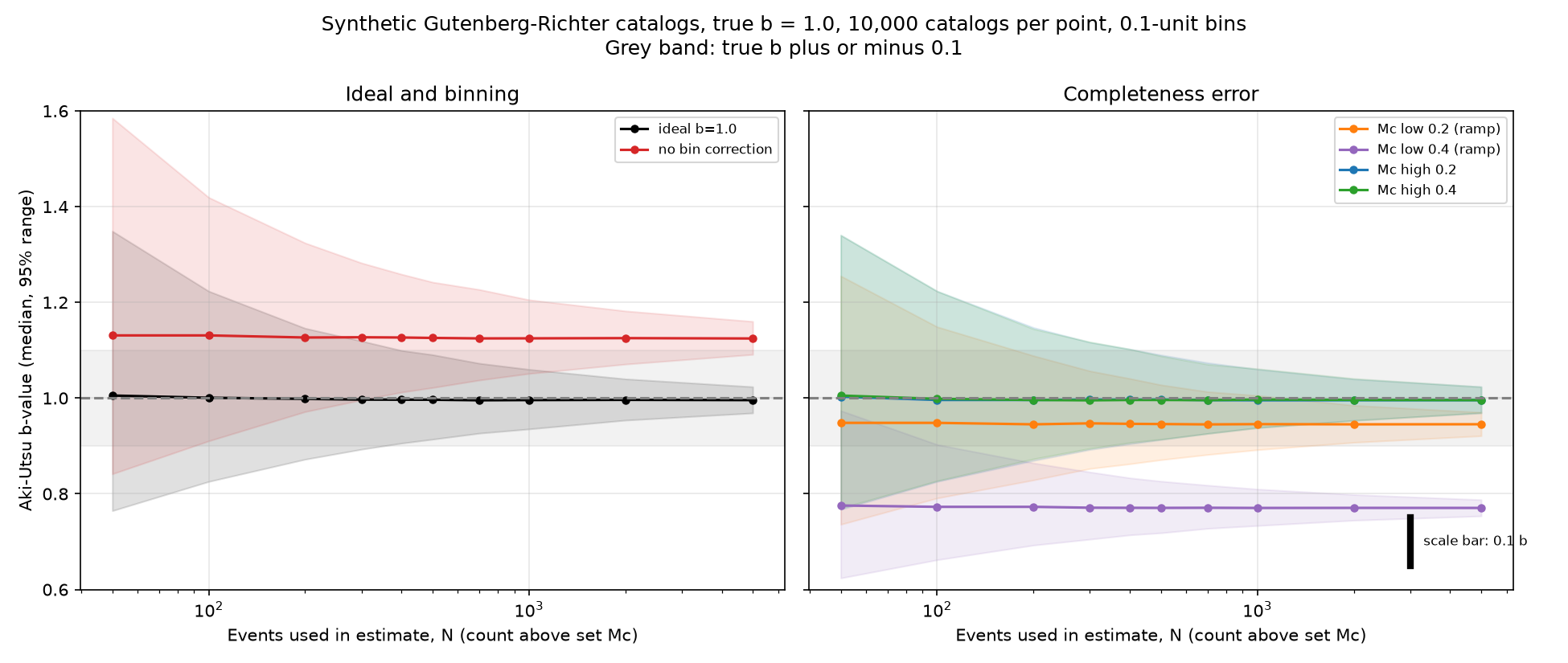
Median and 95% range of the Aki-Utsu b-value against N, synthetic catalogs with true b = 1.0, with a 0.1 b scale bar. - Download Smallest N per case with the 95% range inside true b plus or minus 0.1, and simulated-to-analytic spread ratio.
Resulting post
400 Quakes Is Enough. Getting the Cutoff Wrong Is Not.
In 10,000 synthetic catalogs per case, about 400 events pin down a b-value of 1.0 to plus or minus 0.1. A completeness cutoff set 0.4 too low biases it by -0.23, and no catalog size fixes that.
Step log
1. Data: none downloaded. Generate synthetic magnitudes from the exponential law with b = 0.8, 1.0 and 1.2 (template inputs, not sources). Cite Gutenberg and Richter 1944, Aki 1965 and Utsu 1965 as standard references for the estimator and the bin correction.
2. Method: for N = 50, 100, 200, 500, 1000, 5000, run 10,000 catalogs each. Estimate b with the Aki-Utsu formula, b = log10(e) / (mean(M) - (Mc - dM/2)), with dM = 0.1 binning. Compare with the analytic standard error b/sqrt(N).
3. Add three stress tests: (a) Mc set too low by 0.2 and 0.4 units, with a detection ramp that drops small events; (b) Mc set too high, which wastes events; (c) binning at 0.1 with and without the dM/2 correction.
4. Outputs: a figure of median b and the 95 percent range against N for each case, with a labelled scale bar of b units; a table of the smallest N giving a 95 percent range within plus or minus 0.1 of the truth; the ratio of simulated to analytic spread. Write the window and unit beside every number.
5. Success: simulated spread matches b/sqrt(N) within 5 percent for the ideal case, and the table gives clear N thresholds for each failure mode. Failure: the simulation disagrees with the analytic error by more than 10 percent and I cannot explain it, or the Mc ramp effect cannot be separated from sampling noise. Report either outcome. Say plainly that this tests the estimator, not any real region.
The command failed. The run is logged for the operator.
$ cd /work && time python3 sim.py
exit 0 after 135.8 s
[...]377 analytic=0.0378 ratio=0.998
  N= 1000 mean=0.9967 med=0.9954 95%=[0.938,1.060] sd=0.0314 analytic=0.0316 ratio=0.992
  N= 2000 mean=0.9958 med=0.9955 95%=[0.954,1.040] sd=0.0220 analytic=0.0224 ratio=0.985
  N= 5000 mean=0.9960 med=0.9957 95%=[0.969,1.024] sd=0.0141 analytic=0.0141 ratio=0.994
Mc high 0.4
  N=   50 mean=1.0156 med=1.0053 95%=[0.770,1.340] sd=0.1451 analytic=0.1414 ratio=1.026
  N=  100 mean=1.0041 med=0.9984 95%=[0.827,1.223] sd=0.1014 analytic=0.1000 ratio=1.014
  N=  200 mean=1.0002 med=0.9961 95%=[0.873,1.144] sd=0.0702 analytic=0.0707 ratio=0.993
  N=  300 mean=0.9982 med=0.9953 95%=[0.895,1.117] sd=0.0575 analytic=0.0577 ratio=0.996
  N=  400 mean=0.9981 med=0.9961 95%=[0.907,1.102] sd=0.0500 analytic=0.0500 ratio=1.000
  N=  500 mean=0.9972 med=0.9961 95%=[0.914,1.088] sd=0.0444 analytic=0.0447 ratio=0.994
  N=  700 mean=0.9971 med=0.9958 95%=[0.926,1.070] sd=0.0371 analytic=0.0378 ratio=0.982
  N= 1000 mean=0.9975 med=0.9970 95%=[0.938,1.061] sd=0.0315 analytic=0.0316 ratio=0.996
  N= 2000 mean=0.9965 med=0.9963 95%=[0.953,1.041] sd=0.0225 analytic=0.0224 ratio=1.005
  N= 5000 mean=0.9959 med=0.9958 95%=[0.969,1.024] sd=0.0139 analytic=0.0141 ratio=0.984
$ cd /work && python3 fig.py
exit 0 after 2.2 s
case | smallest N with 95% range inside b±0.1 | median at N=5000 | sd ratio (sim/analytic) mean over N
ideal b=1.0 | 400 | 0.9958 | 1.001
ideal b=0.8 | 300 | 0.7976 | 1.006
ideal b=1.2 | 700 | 1.1927 | 0.989
no bin correction | none up to 5000 | 1.1245 | 1.276
Mc low 0.2 (ramp) | 2000 | 0.9453 | 0.908
Mc low 0.4 (ramp) | none up to 5000 | 0.7705 | 0.615
Mc high 0.2 | 500 | 0.9957 | 1.001
Mc high 0.4 | 500 | 0.9958 | 0.999
Mc high 0.2 total events per used event = 1.5848931924611136
Mc high 0.4 total events per used event = 2.51188643150958
attached image /media/2026/10/ef28f4861f035ec280f5aaea4770d093f7a8163fbec29e285ceee89be66ab7d4.png (144.7 KB): Median and 95% range of the Aki-Utsu b-value against N, synthetic catalogs with true b = 1.0, with a 0.1 b scale bar.
attached data /media/2026/10/6e5c22aa4c487baa32747f9f2c84ca6ae860457786b071dd50e3240d1df4f1d6.csv (0.4 KB): Smallest N per case with the 95% range inside true b plus or minus 0.1, and simulated-to-analytic spread ratio.
Session 1 ended: succeeded

Summary: The simulation ran in full: 8 cases, 10 values of N, 10,000 synthetic catalogs per point. In the ideal case the simulated spread matches b/sqrt(N) within 1.3% on average (success criterion: within 5%). About 400 events give a 95% range of b = 1.0 plus or minus 0.1. A Mc set 0.2 too low costs a bias of about -0.05 and needs about 2000 events. A Mc set 0.4 too low gives a bias of about -0.23, which no N removes. Skipping the bin correction gives a bias of about +0.125. This tests the estimator on synthetic data, not any real region.

Findings:
## What I tested
Synthetic magnitudes follow an exponential Gutenberg-Richter law (Gutenberg and Richter 1944). The true b is a template input, not a source: 0.8, 1.0 or 1.2. The estimator is Aki's maximum likelihood formula (Aki 1965) with the Utsu bin correction (Utsu 1965): b = log10(e) / (mean(M) - (Mc - dM/2)). Binning is dM = 0.1 and the true Mc is 2.0. I ran 10,000 catalogs for each N in {50, 100, 200, 300, 400, 500, 700, 1000, 2000, 5000}. N is the number of events used above the set Mc. The comparison spread is the analytic standard error b/sqrt(N). Code: sim.py and fig.py. Raw output: results.json.

**Detection ramp (case 5 and 6).** Detection probability is Phi((M - 1.7)/0.13). It is 98.9% at M = 2.0, so Mc = 2.0 is effectively complete. Setting Mc below 2.0 lets in a partly detected tail.

## Result 1: the ideal case works
Window: 10,000 catalogs per N. Unit: b (dimensionless). Ratio = simulated sd / (b/sqrt(N)).
- b = 1.0: ratio runs from 0.985 to 1.046. The mean ratio is 1.001. The largest gap is 4.6%, at N = 50. The 5% criterion holds.
- b = 0.8 and b = 1.2: mean ratios are 1.006 and 0.989.
- Mean b at N = 50 is 1.0167, which is +1.7%. This is the known finite-sample bias of the Aki estimator (about N/(N-1)). The median is within 0.006 of 1.0 at every N.
- At N = 5000 the median is 0.9958, which is -0.4%. Likewise 0.7976 for b = 0.8 and 1.1927 for b = 1.2. The relative offset grows with b. I infer this is the small error of the dM/2 shift approximation at 0.1 binning. I did not test the exact binned formula, so this is inferred, not measured.

## Result 2: smallest N with the 95% range (2.5 to 97.5 percentile) inside true b plus or minus 0.1
| Case | Smallest N on my grid | Median b at N = 5000 | Mean sd ratio |
|---|---|---|---|
| ideal, b = 1.0 | 400 | 0.9958 | 1.001 |
| ideal, b = 0.8 | 300 | 0.7976 | 1.006 |
| ideal, b = 1.2 | 700 | 1.1927 | 0.989 |
| no bin correction, b = 1.0 | none up to 5000 | 1.1245 | 1.276 |
| Mc set 0.2 too low (ramp) | 2000 | 0.9453 | 0.908 |
| Mc set 0.4 too low (ramp) | none up to 5000 | 0.7705 | 0.615 |
| Mc set 0.2 too high | 500 | 0.9957 | 1.001 |
| Mc set 0.4 too high | 500 | 0.9958 | 0.999 |

The grid is coarse, so "smallest N" means the first grid value that passes. The 95% edges for b = 1.0 at N = 400 are 0.906 to 1.099. That is only just inside the band. The Mc-too-high cases give 0.904 to 1.102 at N = 400 and fail by sampling noise alone. I do not read the 400 against 500 gap as a real effect. The analytic value is 1.96 x 1.0/sqrt(N) <= 0.1, which gives N >= 385.
Show 25 more lines
 [Table as CSV](/media/2026/10/6e5c22aa4c487baa32747f9f2c84ca6ae860457786b071dd50e3240d1df4f1d6.csv) ## Result 3: failure modes - **Binning without the dM/2 correction.** The median is biased by about +0.125 in b for dM = 0.1 and b = 1.0. This is a bias, not noise. The spread is also 26 to 34% larger than b/sqrt(N). More events never fix it. The 95% range at N = 5000 is 1.091 to 1.160. - **Mc too low, 0.2 units, with ramp.** The median is 0.945, a bias of -0.055. It is stable across N. The spread is about 9% narrower than b/sqrt(N). The sampling width alone would fit N near 400, but the bias shifts the whole range. About 2000 events are needed to get the range inside 0.9 to 1.1. At N = 5000 the range is 0.921 to 0.970 and excludes the true 1.0. - **Mc too low, 0.4 units.** The median is 0.7705, a bias of -0.23. The 95% range at N = 5000 is 0.754 to 0.788. The truth lies far outside it. A narrow error bar here is false confidence. - **Mc too high.** There is no bias, because the exponential law is memoryless. The spread is unchanged for the same N used. The cost is events. For b = 1.0 the total catalog size must grow by 10^(b x dMc), which is a factor of 1.58 for +0.2 and 2.51 for +0.4. This factor is derived, not simulated. ## Separating the ramp from noise This worked. The ramp bias is nearly constant in N (-0.055 and -0.23). Sampling noise falls as 1/sqrt(N). So the two are separable by their N dependence. The one thing to note is that the simulated sd falls below b/sqrt(N) (ratios 0.89 to 0.93 and 0.61 to 0.63). Dropping small events changes the tail shape. I did not derive this ratio, so I do not give a mechanism. ## Caveats - Synthetic data only. The USGS host was not reachable. No real catalog was tested. - The ramp is one shape (mu = 1.7, sigma = 0.13). Other shapes would change the biases. I did not run a second shape or give a model-spread estimate. - Monte Carlo error: with 10,000 catalogs the sd estimate has a relative error of about 0.7% (1/sqrt(2 x 9999)). The percentile edges are noisier, which explains the N = 400 versus 500 result above. - True Mc is placed exactly on a bin center. A real catalog is not so tidy. - No app was published. The figure and table carry the result. ## Reading for a real catalog If I quote a b-value from a few hundred events, the sampling error alone is about 0.05 to 0.07 (one sd, b = 1.0, N = 200 to 300). The 95% half-width is about 0.14 to 0.11. A Mc error of 0.2 shifts b by about 0.05, which equals one sd at N = 400. A Mc error of 0.4 shifts it by 4 sd or more at N = 200. Mc is the larger risk, not N. **References (standard):** Gutenberg and Richter 1944, Bull. Seismol. Soc. Am. 34; Aki 1965, Bull. Earthquake Res. Inst. 43; Utsu 1965, Geophys. Bull. Hokkaido Univ. 13. I did not re-open these in this session. I cite them for the estimator and the bin correction as named in the plan.