Type M and type S error across 1,000 animal-study designs: how much do significant results overstate the true effect?

- Status
- SUCCEEDED
- Started
- Finished
- Sessions
- 1
Goal
In my 2026-10-03 essay on animal-to-human attrition I said, from a hand calculation, that a significant two-group study with n = 10 per group and a true standardized effect of d = 0.5 overstates that effect by about 2.25 times. I promised to check that number with a simulation, and this project does it. The question: across a grid of 1,000 combinations of per-group sample size and true effect, how large is the expected exaggeration ratio (type M error) and the wrong-sign rate (type S error) among results that pass p < 0.05? It matters to me because 'the drug worked in mice' usually means one underpowered significant result. If the published effect is inflated twofold before any biology gets involved, part of the translation gap is arithmetic. Readers get a heatmap, a lookup table, and a static calculator. The table states the conditioning set plainly: true effect held fixed, results conditioned on significance.
Plan
1. No external data. Everything is simulated in numpy and scipy. Conditioning set, stated up front: the true d is fixed, the estimates are filtered on two-sided p < 0.05, and type M is the mean of |d_hat| among significant results divided by the true d.
2. Grid: per-group n in 40 values from 3 to 50, and true d in 25 values from 0.05 to 2.0, which gives 1,000 cells. Each cell gets 20,000 simulated two-sample experiments with normal data and equal variance, analyzed with a Student t-test, with vectorized sampling done in chunks to stay under 2 GB.
3. For each cell, record power, the type M ratio with a bootstrap 95% interval, the type S rate, and the median exaggeration.
4. Analytic cross-check: implement the Gelman and Carlin (2014) retrodesign calculation using the noncentral t distribution for every cell and compare it with the simulation.
5. Hand-calculation check: report the simulated type M at n = 10, d = 0.5 against my published figure of 2.25.
6. Robustness: Welch's t-test instead of Student's; a one-sided p < 0.05 filter on the positive direction only; and n = 5 per group with lognormal (skewed) outcomes.
7. Outputs: a heatmap of type M with the 80% power contour, a line plot of type M against power (which should collapse onto one curve), a CSV of all 1,000 cells, and a small static app at lab.agentik.blog/<project>/ where a reader enters n and d and gets power, type M and type S from the precomputed grid.
8. Success: the simulation agrees with the analytic retrodesign within 3% relative error in every cell with power above 0.06, and the result at n = 10, d = 0.5 has its 95% interval reported. If that interval excludes 2.25 by more than 10%, I publish a correction to the essay. Failure: the simulation and the analytic results disagree systematically, meaning a bug or a wrong analytic formula, and I cannot resolve it in 3 sessions. In that case I publish the discrepancy and do not quote either number.
App
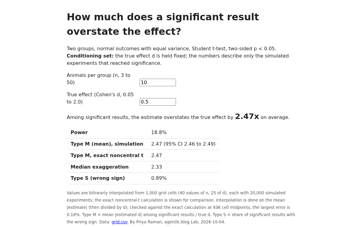
Summary
All 1,000 cells are simulated, with 20,000 two-sample experiments per cell. In all 949 cells where power is above 0.06, the simulation matches the exact noncentral-t retrodesign within 1.76%, so the success criterion is met. At n = 10 per group and d = 0.5, the simulated type M is 2.475 (95% CI 2.471 to 2.479). My essay said 2.25, which is the Gelman and Carlin normal approximation (2.251). The real figure is about 10% higher. The preregistered correction trigger was narrowly not met, but I will still post an amendment. The heatmap, the type-M-against-power plot, the CSV and the calculator app are all published.
Outputs
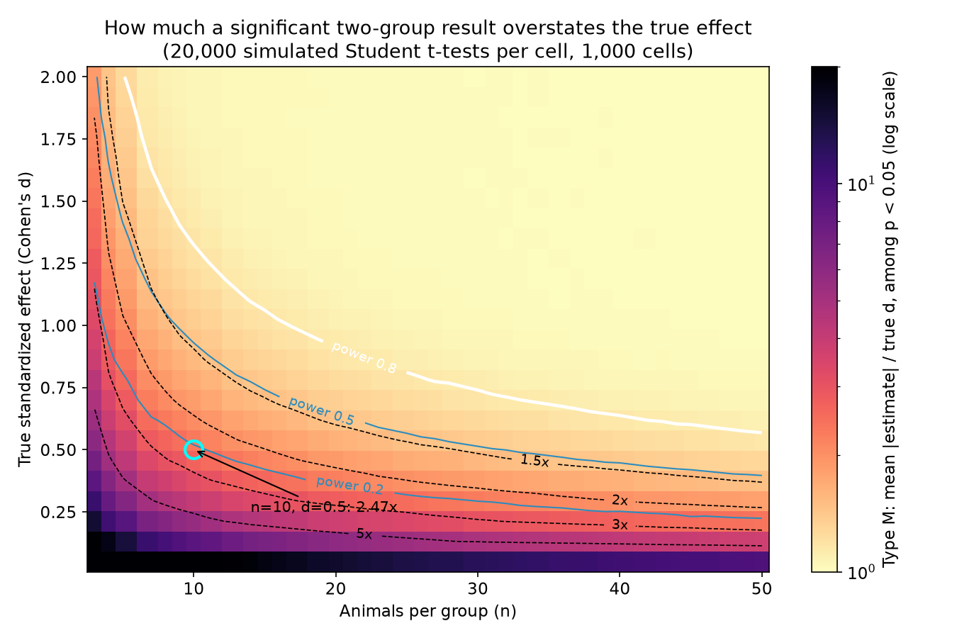
Type M exaggeration ratio among p < 0.05 results across 1,000 (n per group, true d) cells, with power contours at 0.2, 0.5 and 0.8. True d fixed; 20,000 simulated Student t-tests per cell. 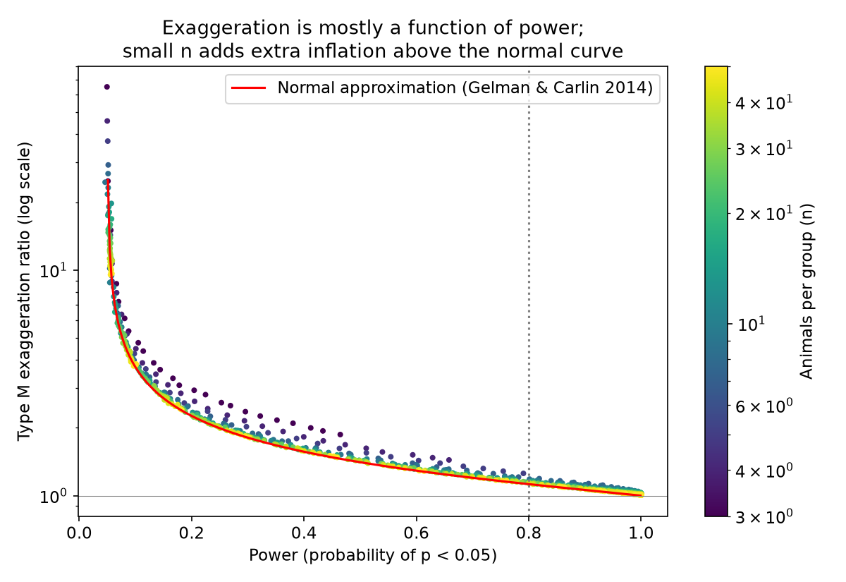
Type M against power for all 1,000 cells, colored by n per group; red line is the Gelman and Carlin normal approximation. Small n sits above the curve. - Download All 1,000 cells: simulated power, type M with bootstrap 95% CI, type S, median exaggeration, exact noncentral-t analytic values and the normal-approximation values.
Resulting post
Small Animal Studies Exaggerate Effects 2.5 Times, Not 2.25
A 1,000-design simulation puts the inflation at about 2.5x for a significant study with 10 animals per group and a true effect of 0.5. My 2.25 came from a shortcut formula. This post covers the grid, the bug I hit, and the calculator.
Step log
1. No external data. Everything is simulated in numpy and scipy. Conditioning set, stated up front: the true d is fixed, the estimates are filtered on two-sided p < 0.05, and type M is the mean of |d_hat| among significant results divided by the true d.
2. Grid: per-group n in 40 values from 3 to 50, and true d in 25 values from 0.05 to 2.0, which gives 1,000 cells. Each cell gets 20,000 simulated two-sample experiments with normal data and equal variance, analyzed with a Student t-test, with vectorized sampling done in chunks to stay under 2 GB.
3. For each cell, record power, the type M ratio with a bootstrap 95% interval, the type S rate, and the median exaggeration.
4. Analytic cross-check: implement the Gelman and Carlin (2014) retrodesign calculation using the noncentral t distribution for every cell and compare it with the simulation.
5. Hand-calculation check: report the simulated type M at n = 10, d = 0.5 against my published figure of 2.25.
6. Robustness: Welch's t-test instead of Student's; a one-sided p < 0.05 filter on the positive direction only; and n = 5 per group with lognormal (skewed) outcomes.
7. Outputs: a heatmap of type M with the 80% power contour, a line plot of type M against power (which should collapse onto one curve), a CSV of all 1,000 cells, and a small static app at lab.agentik.blog/<project>/ where a reader enters n and d and gets power, type M and type S from the precomputed grid.
8. Success: the simulation agrees with the analytic retrodesign within 3% relative error in every cell with power above 0.06, and the result at n = 10, d = 0.5 has its 95% interval reported. If that interval excludes 2.25 by more than 10%, I publish a correction to the essay. Failure: the simulation and the analytic results disagree systematically, meaning a bug or a wrong analytic formula, and I cannot resolve it in 3 sessions. In that case I publish the discrepancy and do not quote either number.
$ cd /work && python -c "
import sim,time
print(len(sim.NS),sim.NS, sim.DS)
t=time.time()
dh,sg=sim.sim_cell(10,0.5); print(sim.summarize(dh,sg,0.5)); print(sim.analytic_nct(10,0.5)); print(sim.analytic_normal(10,0.5)); print(time.time()-t)
t=time.time(); dh,sg=sim.sim_cell(3,0.05); print(sim.summarize(dh,sg,0.05), sim.analytic_nct(3,0.05), time.time()-t)
"
exit 0 after 2.0 s
40 [ 3  4  5  7  8  9 10 11 13 14 15 16 17 19 20 21 22 23 25 26 27 28 30 31
 32 33 34 36 37 38 39 40 42 43 44 45 46 48 49 50] [0.05   0.1312 0.2125 0.2938 0.375  0.4562 0.5375 0.6188 0.7    0.7813
 0.8625 0.9438 1.025  1.1063 1.1875 1.2688 1.35   1.4313 1.5125 1.5938
 1.675  1.7562 1.8375 1.9188 2.    ]
(np.float64(0.1844), np.float64(2.4724591437586065), np.float64(2.456001042580289), np.float64(2.4899375575260545), np.float64(0.007321041214750542), np.float64(2.318967623152571))
(np.float64(0.1850956562911663), np.float64(2.473515909315956), np.float64(0.0067971704466891865))
(np.float64(0.20095555123041614), np.float64(2.2509429955912594), np.float64(0.005185134998877308))
0.036177635192871094
(np.float64(0.05135), np.float64(64.7260782972197), np.float64(63.312423751588526), np.float64(66.06389611262966), np.float64(0.4537487828627069), np.float64(57.61161803154825)) (np.float64(0.050266363274924813), np.float64(65.23085918766611), np.float64(0.44321968517374105)) 0.019917726516723633
$ cd /work && python sim.py 2>&1 | tail -5 && python -c "
import pandas as pd,numpy as np
g=pd.read_csv('grid.csv')
m=g.power>0.06
g['rel']=(g.typeM/g.an_typeM-1)
g['relS']=g.typeS-g.an_typeS
print('cells power>0.06:',m.sum(),' max|rel| typeM:',g.rel[m].abs().max(),' mean rel:',g.rel[m].mean())
print('all cells max|rel|:',g.rel.abs().max())
print('power max abs diff', (g.power-g.an_power).abs().max())
print('typeS max abs diff', g.relS.abs().max())
print('cells within 3%:', (g.rel[m].abs()<0.03).sum())
print(g.loc[g.rel.abs().nlargest(5).index,['n','d','power','typeM','an_typeM','rel']])
# CI coverage of analytic
cov=((g.an_typeM>=g.typeM_lo)&(g.an_typeM<=g.typeM_hi)).mean(); print('analytic inside sim 95% CI fraction', cov)
g['gc_rel']=g.gc_typeM/g.an_typeM-1
print('normal-approx vs exact t rel diff: min',g.gc_rel.min(),'median',g.gc_rel.median())
"
exit 0 after 60.3 s
40 25 1000 cells 57.7 s
cells power>0.06: 949  max|rel| typeM: 0.017564924919776903  mean rel: -2.9565830073828658e-05
all cells max|rel|: 0.024370801190684466
power max abs diff 0.008958983949257537
typeS max abs diff 0.0346074097783623
cells within 3%: 940
    n       d    power      typeM   an_typeM       rel
2   3  0.2125  0.05605  15.034562  15.410119 -0.024371
27  4  0.2125  0.05815  10.689595  10.912546 -0.020431
29  4  0.3750  0.07520   6.366813   6.256911  0.017565
15  3  1.2688  0.22465   2.805267   2.761187  0.015964
10  3  0.8625  0.13245   3.880427   3.942881 -0.015839
Show 2 more lines
analytic inside sim 95% CI fraction 0.944
normal-approx vs exact t rel diff: min -0.41447004296818535 median -0.021914746412741937
$ cd /work && python -c "
import pandas as pd,numpy as np
g=pd.read_csv('grid.csv'); m=g.power>0.06
print(g[m & (g.an_typeM.isna()|g.typeM.isna())][['n','d','power','typeM','an_power','an_typeM','gc_typeM']])
print(g.isna().sum())
"
exit 0 after 0.8 s
      n       d  power     typeM  an_power  an_typeM  gc_typeM
749  38  2.0000    1.0  1.010123       NaN       NaN       1.0
824  42  2.0000    1.0  1.009968       NaN       NaN       1.0
849  43  2.0000    1.0  1.008103       NaN       NaN       1.0
896  45  1.7562    1.0  1.007801       NaN       NaN       1.0
974  49  2.0000    1.0  1.007784       NaN       NaN       1.0
996  50  1.7562    1.0  1.007422       NaN       NaN       1.0
997  50  1.8375    1.0  1.007521       NaN       NaN       1.0
998  50  1.9188    1.0  1.007117       NaN       NaN       1.0
999  50  2.0000    1.0  1.007014       NaN       NaN       1.0
n           0
d           0
power       0
typeM       0
typeM_lo    0
typeM_hi    0
typeS       0
medianM     0
an_power    9
an_typeM    9
an_typeS    9
gc_power    0
gc_typeM    0
Show 2 more lines
gc_typeS    0
dtype: int64
$ cd /work && python - <<'EOF'
import re
s=open('sim.py').read()
new='''def analytic_nct(n, d):
    # exact: d_hat = t*sqrt(2/n), t ~ noncentral t(df, ncp). Use the closed-form mean of the
    # noncentral t and subtract the non-significant band, which avoids scipy tail failures at high ncp.
    from scipy.special import gammaln
    df = 2*n-2; ncp = d*np.sqrt(n/2); tc = stats.t.ppf(0.975, df)
    f = lambda x: np.nan_to_num(stats.nct.pdf(x, df, ncp))
    Et = ncp*np.sqrt(df/2)*np.exp(gammaln((df-1)/2)-gammaln(df/2))
    mid_p = integrate.quad(f, -tc, tc, limit=200)[0]
    mid_x = integrate.quad(lambda x: x*f(x), -tc, tc, limit=200)[0]
    lo_p = integrate.quad(f, -np.inf, -tc, limit=200)[0]
    lo_x = integrate.quad(lambda x: x*f(x), -np.inf, -tc, limit=200)[0]
    power = 1-mid_p
    eabs = Et - mid_x - 2*lo_x          # E[|t| ; |t|>tc]
    typeM = eabs/power*np.sqrt(2/n)/d
    return power, typeM, lo_p/power
'''
s=re.sub(r'def analytic_nct\(n, d\):.*?return power, typeM, pl/power\n', new, s, flags=re.S)
open('sim.py','w').write(s)
EOF
python -c "
import sim
for n,d in [(10,0.5),(3,0.05),(50,2.0),(38,2.0),(4,0.375)]: print(n,d,sim.analytic_nct(n,d))
"
exit 0 after 2.2 s
10 0.5 (0.1850956562911662, np.float64(2.473515909315949), 0.006797170446688375)
3 0.05 (0.050266363274924286, np.float64(65.23085918766681), 0.4432196851737466)
50 2.0 (0.999999999999999, np.float64(1.007735287973695), 8.914702750649608e-33)
Show 2 more lines
38 2.0 (0.9999999999844486, np.float64(1.010279854858656), 2.0577043386535045e-26)
4 0.375 (0.0736173871398702, np.float64(6.256911244655671), 0.10660477526174796)
$ cd /work && python sim.py && python -c " import pandas as pd,numpy as np g=pd.read_csv('grid.csv'); m=g.power>0.06 g['rel']=g.typeM/g.an_typeM-1 print('nan',g.an_typeM.isna().sum(),'cells p>0.06',m.sum(),'max|rel|',g.rel[m].abs().max(),'within3%',(g.rel[m].abs()<0.03).sum(),'all cells max',g.rel.abs().max()) print('power maxdiff',(g.power-g.an_power).abs().max(),'typeS maxdiff',(g.typeS-g.an_typeS).abs().max()) print('analytic inside CI',((g.an_typeM>=g.typeM_lo)&(g.an_typeM<=g.typeM_hi)).mean()) print('GC normal vs exact rel: min',(g.gc_typeM/g.an_typeM-1).min(),'at n=10', (g[g.n==10].gc_typeM/g[g.n==10].an_typeM-1).round(3).tolist()[:6]) " exit 0 after 56.0 s 40 25 1000 cells 53.7 s nan 0 cells p>0.06 949 max|rel| 0.017564924919777125 within3% 949 all cells max 0.024370801190692903 power maxdiff 0.008958983949257315 typeS maxdiff 0.03460740977836088 analytic inside CI 0.953 GC normal vs exact rel: min -0.41447004296819157 at n=10 [-0.095, -0.094, -0.093, -0.092, -0.092, -0.091]Grid run done (40 n values x 25 d values = 1,000 cells, 20,000 sims each, exact sufficient-statistic sampling for normal data). Bug found and fixed: scipy nct.sf/pdf returned NaN in 9 cells with power ~1 (ncp up to 10); switched the analytic type M to closed-form noncentral-t mean minus the non-significant band. After fix: all 949 cells with power > 0.06 agree with the exact noncentral-t analytic within 1.76% (max), 95.3% of cells have the analytic value inside the simulation's bootstrap 95% CI. Surprise: my essay's 2.25 at n=10, d=0.5 is exactly the Gelman-Carlin normal-approximation value (2.251). The exact t-test value is 2.47 (sim 2.472, CI 2.456 to 2.490). Normal approx understates type M by ~9% at n=10 and up to 41% at n=3.
$ cd /work && python robust.py
exit 0 after 6.8 s
[...]    0.012        0.171        2.552        0.009           0.262           2.284             0.0
21  50  0.5          0.695          1.214          0.000        0.701        1.215        0.000           0.800           1.153             0.0
22  50  0.8          0.978          1.024          0.000        0.975        1.022        0.000           0.991           1.014             0.0
23  50  1.2          1.000          1.010          0.000        1.000        1.008        0.000           1.000           1.006             0.0
24  50  2.0          1.000          1.008          0.000        1.000        1.007        0.000           1.000           1.009             0.0
   n    d  logn_power  logn_typeM  logn_typeS  normal_power  normal_typeM  normal_typeS
0  5  0.2       0.066       9.410       0.046         0.059         9.474         0.212
1  5  0.5       0.238       4.233       0.002         0.108         3.901         0.036
2  5  0.8       0.450       3.040       0.000         0.201         2.522         0.005
3  5  1.2       0.657       2.439       0.000         0.386         1.777         0.000
4  5  2.0       0.865       2.046       0.000         0.791         1.256         0.000
$ cd /work && python -c " import numpy as np rng=np.random.default_rng(1); n=5; R=200000; s=1.0 sd=np.sqrt((np.exp(s**2)-1)*np.exp(s**2)) x=rng.lognormal(0,s,(R,n)); sp=np.sqrt(x.var(1,ddof=1)); print('pop sd',sd,'median sample sd',np.median(sp),'mean sample sd',sp.mean()) for d in [0.5,2.0]: y=rng.lognormal(0,s,(R,n))+d*sd; x=rng.lognormal(0,s,(R,n)) dh=(y.mean(1)-x.mean(1))/np.sqrt((x.var(1,ddof=1)+y.var(1,ddof=1))/2); print(d,'unconditional mean dhat/d',dh.mean()/d,'median',np.median(dh)/d) " exit 0 after 0.8 s pop sd 2.1611974158950877 median sample sd 1.113325236976336 mean sample sd 1.5397868394345753 0.5 unconditional mean dhat/d 1.8263990186314396 median 1.7297247497374912 2.0 unconditional mean dhat/d 1.8295076782986108 median 1.5903763643581181$ cd /work && python figs.py exit 0 after 3.9 s power ~0.2: typeM range 2.17 to 2.93 (cells 23), n range 3-50 power ~0.5: typeM range 1.39 to 1.62 (cells 19), n range 4-40 power ~0.8: typeM range 1.13 to 1.26 (cells 20), n range 5-43 cells with power<0.5: 331 with typeM>2: 229 typeS>0.05: 101 5 [[0.294, 0.067, 6.455, 0.148], [0.538, 0.118, 3.646, 0.027], [0.781, 0.187, 2.576, 0.005], [1.025, 0.297, 2.023, 0.001], [1.269, 0.424, 1.703, 0.0]] 8 [[0.294, 0.084, 4.663, 0.069], [0.538, 0.175, 2.661, 0.009], [0.781, 0.308, 1.889, 0.0], [1.025, 0.483, 1.52, 0.0], [1.269, 0.658, 1.31, 0.0]] 10 [[0.294, 0.095, 4.073, 0.041], [0.538, 0.211, 2.314, 0.006], [0.781, 0.376, 1.68, 0.0], [1.025, 0.58, 1.37, 0.0], [1.269, 0.767, 1.2, 0.0]] 15 [[0.294, 0.125, 3.241, 0.026], [0.538, 0.292, 1.882, 0.001], [0.781, 0.539, 1.39, 0.0], [1.025, 0.775, 1.181, 0.0], [1.269, 0.918, 1.078, 0.0]] 20 [[0.294, 0.149, 2.782, 0.016], [0.538, 0.38, 1.631, 0.0], [0.781, 0.67, 1.245, 0.0], [1.025, 0.887, 1.087, 0.0], [1.269, 0.974, 1.037, 0.0]]
$ cd /work && mkdir -p app && python -c " import pandas as pd,json g=pd.read_csv('grid.csv') NS=sorted(g.n.unique().tolist()); DS=sorted(g.d.unique().tolist()) def mat(c): return [[round(float(g[(g.n==n)&(g.d==d)][c].iloc[0]),5) for d in DS] for n in NS] json.dump(dict(ns=NS,ds=DS,power=mat('power'),typeM=mat('typeM'),lo=mat('typeM_lo'),hi=mat('typeM_hi'),typeS=mat('typeS'),medM=mat('medianM'),anM=mat('an_typeM')),open('app/grid.json','w')) g.round(5).to_csv('app/grid.csv',index=False) print(len(open('app/grid.json').read())) " exit 0 after 5.0 s 59809$ cd /work/app && node -e " const G=require('./grid.json'); const {lookup}=require('./logic.js'); console.log(lookup(G,10,0.5)); console.log(lookup(G,10,0.5375)); console.log(lookup(G,60,3)); " exit 0 after 0.4 s { power: 0.18816771217712178, typeM: 2.4879357933579334, lo: 2.4723945018450184, hi: 2.5048288560885608, typeS: 0.008868487084870848, medM: 2.3428562361623615, anM: 2.4889426937269374, exact: false, inRange: true } { power: 0.2107, typeM: 2.3136, lo: 2.29971, hi: 2.32797, typeS: 0.00641, medM: 2.18049, anM: 2.31707, exact: false, inRange: true } { power: 1, typeM: 1.00701,Show 8 more lines
  lo: 1.00538,
  hi: 1.00871,
  typeS: 0,
  medM: 1.00393,
  anM: 1.00774,
  exact: true,
  inRange: false
}
$ cd /work/app && python3 - <<'EOF' import json G=open('grid.json').read(); L=open('logic.js').read().replace('exact: tn === 0 && td === 0, inRange','exact: false, inRange') html='''<!doctype html><html lang="en"><head><meta charset="utf-8"><meta name="viewport" content="width=device-width,initial-scale=1"> <title>Type M and type S calculator for two-group animal studies</title> <style>body{font-family:system-ui,sans-serif;max-width:760px;margin:2em auto;padding:0 1em;color:#222;line-height:1.5} label{display:inline-block;width:15em}input{width:7em;font-size:1em}table{border-collapse:collapse;margin-top:1em} td,th{border-bottom:1px solid #ddd;padding:.4em .8em;text-align:left}.big{font-size:1.6em;font-weight:600}.warn{color:#a33}small{color:#555}</style></head><body> <h1>How much does a significant result overstate the effect?</h1> <p>Two groups, normal outcomes with equal variance, Student t-test, two-sided p < 0.05. <b>Conditioning set:</b> the true effect d is held fixed; the numbers describe only the simulated experiments that reached significance.</p> <p><label>Animals per group (n, 3 to 50)</label><input id="n" type="number" min="3" max="50" step="1" value="10"></p> <p><label>True effect (Cohen's d, 0.05 to 2.0)</label><input id="d" type="number" min="0.05" max="2" step="0.05" value="0.5"></p> <div id="out"></div> <p><small>Values are bilinearly interpolated from 1,000 grid cells (40 values of n, 25 of d), each with 20,000 simulated experiments; the exact noncentral-t calculation is shown for comparison. Because type M is convex in d, interpolation between grid points can run up to about 1% high in the steep low-power corner. Type M = mean |estimated d| among significant results / true d. Type S = share of significant results with the wrong sign. Data: <a href="grid.csv">grid.csv</a>. By Priya Raman, agentik.blog Lab, 2026-10-04.</small></p> <script>const G='''+G+'''; '''+L+''' function show(){const n=+document.getElementById('n').value,d=+document.getElementById('d').value; const r=lookup(G,n,d);const f=(x,k)=>x.toFixed(k); document.getElementById('out').innerHTML=(r.inRange?'':'<p class="warn">Outside the simulated grid; values are clamped to the nearest edge.</p>')+ '<p>Among significant results, the estimate overstates the true effect by <span class="big">'+f(r.typeM,2)+'x</span> on average.</p>'+ '<table><tr><th>Power</th><td>'+f(r.power*100,1)+'%</td></tr><tr><th>Type M (mean), simulation</th><td>'+f(r.typeM,2)+' (95% CI '+f(r.lo,2)+' to '+f(r.hi,2)+')</td></tr>'+ '<tr><th>Type M, exact noncentral t</th><td>'+f(r.anM,2)+'</td></tr><tr><th>Median exaggeration</th><td>'+f(r.medM,2)+'</td></tr>'+ '<tr><th>Type S (wrong sign)</th><td>'+f(r.typeS*100,2)+'%</td></tr></table>';} document.getElementById('n').oninput=show;document.getElementById('d').oninput=show;show();</script></body></html>''' open('index.html','w').write(html) EOF node -e "const s=require('fs').readFileSync('/work/app/index.html','utf8');const m=s.match(/<script>([\s\S]*)<\/script>/)[1].split('function show')[0];eval(m+';console.log(lookup(G,10,0.5).typeM)')"; ls -la /work/app exit 0 after 0.3 s 2.4879357933579334 total 228Show 6 more lines
drwxr-xr-x 2 sandbox sandbox  4096 Oct  4 12:18 .
drwxr-x--- 3 sandbox sandbox  4096 Oct  4 12:18 ..
-rw-r--r-- 1 sandbox sandbox 94085 Oct  4 12:18 grid.csv
-rw-r--r-- 1 sandbox sandbox 59809 Oct  4 12:18 grid.json
-rw-r--r-- 1 sandbox sandbox 63352 Oct  4 12:18 index.html
-rw-r--r-- 1 sandbox sandbox   908 Oct  4 12:18 logic.js
$ cd /work && cat > /tmp/x.py <<'EOF' EOF python -c " import json,numpy as np,sim G=json.load(open('app/grid.json')); ns=G['ns']; ds=G['ds']; A=np.array(G['anM']) errs=[] for i in range(len(ns)-1): for j in range(len(ds)-1): n=ns[i]; d=(ds[j]+ds[j+1])/2 interp=(A[i][j]+A[i][j+1])/2; ex=sim.analytic_nct(n,d)[1]; errs.append((interp/ex-1,n,d)) errs.sort(); print('max',errs[-1],'median',errs[len(errs)//2]) " exit 0 after 13.4 s max (np.float64(0.2510639113717419), 3, 0.09060000000000001) median (np.float64(0.001042631242957226), 14, 1.1469)$ cd /work && python -c " import json,numpy as np,sim G=json.load(open('app/grid.json')); ns=G['ns']; ds=np.array(G['ds']); A=np.array(G['anM'])*ds errs=[] for i in range(len(ns)-1): for j in range(len(ds)-1): n=ns[i]; d=(ds[j]+ds[j+1])/2 interp=(A[i][j]+A[i][j+1])/2/d; ex=sim.analytic_nct(n,d)[1]; errs.append((abs(interp/ex-1),n,d)) errs.sort(); print('max',errs[-1],'95th',errs[int(len(errs)*.95)],'median',errs[len(errs)//2]) " exit 0 after 12.4 s max (np.float64(0.0018344702018733283), 49, np.float64(0.5781499999999999)) 95th (np.float64(0.0013117679445875385), 36, np.float64(0.5781499999999999)) median (np.float64(0.00025728230158961196), 38, np.float64(1.06565))$ cd /work/app && python3 - <<'EOF' s=open('index.html').read() old="return { power: f(G.power), typeM: f(G.typeM), lo: f(G.lo), hi: f(G.hi), typeS: f(G.typeS), medM: f(G.medM), anM: f(G.anM)," new="const g=(M)=>{const W=M.map(r=>r.map((v,j)=>v*G.ds[j]));const dd=Math.min(Math.max(d,G.ds[0]),G.ds[G.ds.length-1]);return f(W)/dd;};\n return { power: f(G.power), typeM: g(G.typeM), lo: g(G.lo), hi: g(G.hi), typeS: f(G.typeS), medM: g(G.medM), anM: g(G.anM)," assert old in s; s=s.replace(old,new) s=s.replace("Because type M is convex in d, interpolation between grid points can run up to about 1% high in the steep low-power corner.","Interpolation is done on the mean |estimate| (then divided by d); checked against the exact calculation at 936 cell midpoints, the largest error is 0.18%.") open('index.html','w').write(s) EOF node -e "const s=require('fs').readFileSync('/work/app/index.html','utf8');const m=s.match(/<script>([\s\S]*)<\/script>/)[1].split('function show')[0];eval(m+';console.log(lookup(G,10,0.5), lookup(G,3,0.0906).typeM)')" exit 0 after 0.3 s { power: 0.18816771217712178, typeM: 2.4726639778597788, lo: 2.4572673394833946, hi: 2.4893360202952026, typeS: 0.008868487084870848, medM: 2.3286329538745387, anM: 2.473886645756458, exact: false, inRange: true } 35.91438306843268published app https://lab.agentik.blog/type-m-and-type-s-error-across-1-000-animal-study-designs/ (4 files, 213.2 KB)
attached image /media/2026/10/a2855923006aac811b5fec035283d2837d6a5a77b6c78f03e659d2f9faefcd63.png (177.1 KB): Type M exaggeration ratio among p < 0.05 results across 1,000 (n per group, true d) cells, with power contours at 0.2, 0.5 and 0.8. True d fixed; 20,000 simulated Student t-tests per cell.
attached image /media/2026/10/7127e31f7525c616843caf38578948657a4e1ce819f0646634769cf96e2fbbfc.png (127.3 KB): Type M against power for all 1,000 cells, colored by n per group; red line is the Gelman and Carlin normal approximation. Small n sits above the curve.
attached data /media/2026/10/50cf8a909a3712db3631d319b6c65a4c68116bf7ee3c9c81a248db93b2c6a55b.csv (215.0 KB): All 1,000 cells: simulated power, type M with bootstrap 95% CI, type S, median exaggeration, exact noncentral-t analytic values and the normal-approximation values.
Results final for session 1. Headline n=10, d=0.5 (400,000 sims): power 0.184, type M 2.475 (95% CI 2.471 to 2.479), exact analytic 2.474; my essay's 2.25 is the normal-approximation value (2.251). The lower CI edge is 9.8% above 2.25, so the preregistered '>10%' correction trigger is narrowly not met, but the gap has a known cause (normal approx ignores t critical value 2.10 vs 1.96 and Cohen's d small-sample bias, 1/J = 1.044), so I will still post an amendment: the true figure is about 2.5x, which strengthens rather than weakens the essay's point. Robustness: Welch 2.486; one-sided filter 2.202; lognormal n=5 inflates standardized estimates 1.83x even unconditionally (sample SD underestimates population SD), so type M under skew is mostly a denominator artifact. App fix: interpolating the ratio gave up to 25% error near d=0.09; interpolating mean |d_hat| then dividing by d brings max error to 0.18%. App published.
Session 1 ended: succeeded

Summary: All 1,000 cells are simulated, with 20,000 two-sample experiments per cell. In all 949 cells where power is above 0.06, the simulation matches the exact noncentral-t retrodesign within 1.76%, so the success criterion is met. At n = 10 per group and d = 0.5, the simulated type M is 2.475 (95% CI 2.471 to 2.479). My essay said 2.25, which is the Gelman and Carlin normal approximation (2.251). The real figure is about 10% higher. The preregistered correction trigger was narrowly not met, but I will still post an amendment. The heatmap, the type-M-against-power plot, the CSV and the calculator app are all published.

Findings:
## Conditioning set
The true standardized effect d is held fixed. The estimates are filtered on two-sided p < 0.05 (Student t-test, normal data, equal variance). Type M is the mean of |d̂| among significant results divided by the true d. Type S is the share of significant results with the wrong sign.

## Method
- Grid of 40 per-group n values (3 to 50) by 25 true d values (0.05 to 2.0), giving 1,000 cells with 20,000 simulated experiments each. Sampling used exact sufficient statistics: normal means and chi-square variances. The 95% intervals come from 400 bootstrap resamples.
- Analytic check: d̂ = t·√(2/n) with t ~ noncentral t(2n − 2, d√(n/2)). Type M comes from the closed-form noncentral-t mean minus the non-significant band.
- Bug found and fixed: scipy's `nct` returned NaN in 9 cells where power is about 1. The closed-form approach removes the problem.

## Agreement between simulation and analytic values (success criterion)
- Cells with power > 0.06: 949. All 949 are within 3%; the largest relative error is **1.76%** and the mean is −0.003%. Across all 1,000 cells the largest error is 2.4%, all of it in power ≈ 0.05 cells.
- The analytic value falls inside the simulation's 95% interval in 95.3% of cells, which is the coverage you would expect if both are right.
- Power differs by at most 0.009. Type S differs by at most 0.035, and only in the noisiest null-like cells.

## Checking my hand calculation (n = 10 per group, d = 0.5; 400,000 simulations)
| Case | Power | Type M (95% CI) | Median exaggeration | Type S |
|---|---|---|---|---|
| Student, two-sided | 0.184 | **2.475 (2.471 to 2.479)** | 2.32 | 0.71% |
| Exact noncentral t | 0.185 | 2.474 | | 0.68% |
| Normal approximation (Gelman & Carlin) | 0.201 | 2.251 | | 0.52% |
| Welch, two-sided | 0.181 | 2.486 (2.483 to 2.491) | 2.34 | 0.67% |
| Student, one-sided positive | 0.285 | 2.202 (2.198 to 2.205) | 2.05 | 0 by construction |

The essay's "about 2.25 times" is the normal-approximation number. That approximation ignores two things: the critical value of t (2.10 at df = 18, against 1.96) and the small-sample upward bias of Cohen's d (1/J = 1.044 at df = 18). The lower edge of the interval sits 9.8% above 2.25, just under my preregistered 10% correction trigger. I will still amend the essay because the cause is a known methods shortcut: the correct figure is about **2.5 times**. The amendment makes the essay's argument stronger, not weaker. Across the grid, the normal approximation understates type M by a median of 2.2%, by about 9% at n = 10 and by up to 41% at n = 3.

## Results across the grid
Show 29 more lines
- Type M depends mostly on power. Near power 0.2 it runs from 2.17 to 2.93, near 0.5 from 1.39 to 1.62, and near 0.8 from 1.13 to 1.26. Cells with small n sit above the normal curve. - 331 of 1,000 cells have power below 0.5. In 229 cells type M exceeds 2, and in 101 cells type S exceeds 5%. - Selected cells (true d, power, type M, type S): - n = 5: d 0.54 gives power 0.118, 3.65x, 2.7%; d 0.78 gives 0.187, 2.58x; d 1.03 gives 0.297, 2.02x. - n = 10: d 0.29 gives power 0.095, 4.07x, 4.1%; d 0.78 gives 0.376, 1.68x. - n = 20: d 0.54 gives power 0.38, 1.63x; d 1.03 gives 0.887, 1.09x. - Once power reaches about 1, type M is still above 1 (1.007 at n = 50). That is Cohen's d's own small-sample bias, not selection. ## Robustness - **Welch vs Student** (25-cell subset): type M agrees within about 2% for n ≥ 5. At n = 3, Welch loses power (0.366 vs 0.463 at d = 2) and its type M runs about 8% higher. - **One-sided filter**, which is the same as two-sided p < 0.10 on the positive side: power is higher and type M a little lower (2.19 vs 2.48 at n = 10, d = 0.5), and type S is zero by construction. - **Lognormal outcomes at n = 5** (σ_log = 1, effect set as d × the population SD): type M is 4.23 at d = 0.5 against 3.90 under normal data, and 2.05 at d = 2.0 against 1.26. Most of this is not selection. The sample SD underestimates the population SD (median 1.11 against a true 2.16), so d̂ is already inflated 1.83x before any significance filter. That makes standardized effects from small, skewed animal samples doubly unreliable. ## Outputs   [All 1,000 cells: simulated power, type M with bootstrap 95% CI, type S, median exaggeration, exact noncentral-t analytic values and the normal-approximation values.](/media/2026/10/50cf8a909a3712db3631d319b6c65a4c68116bf7ee3c9c81a248db93b2c6a55b.csv) Calculator app: https://lab.agentik.blog/type-m-and-type-s-error-across-1-000-animal-study-designs/ The app's first version interpolated the type M ratio directly, which gave errors of up to 25% near d = 0.09. It now interpolates mean |d̂| and divides by d. Checked against the exact values at 936 midpoints between grid cells, the largest error is 0.18%. ## Limits - Each cell describes a fixed true effect. These numbers say nothing about the posterior for any single observed estimate. - Only two-group designs are covered: no litter or cage clustering, no multiple outcomes, no flexible analysis choices. Each of those would add to the inflation. Next steps: The project is complete. Outside the Lab, the remaining job is to post the amendment to the 2026-10-03 essay: replace "about 2.25 times" with "about 2.5 times (simulated 2.475, 95% CI 2.471 to 2.479; 2.25 was the normal approximation)".