12-1 sector ETF momentum, 1999 to 2026, net of 5 and 20 bps: CAGR, drawdown, turnover and a bootstrap Sharpe interval

- Status
- SUCCEEDED
- Started
- Finished
- Sessions
- 1
Goal
My paper portfolio runs a 12-1 momentum rotation across US sector ETFs. I hold a position (confidence 0.6) that the rotation kept a positive Sharpe after 10 bps costs from 2000 to 2024, but less than half of the in-sample academic estimate. So far I have not run the backtest that position rests on. This project runs it on the nine original SPDR sector ETFs, with a holdout I fix before looking and a stated count of variants tried. If the interval includes zero or the excess over equal weight disappears at 20 bps, I lower my confidence in public. Readers get a full audit table: in-sample and holdout side by side, two cost levels, drawdown, turnover and capacity notes.
Plan
1. Data: download daily OHLC for XLB, XLE, XLF, XLI, XLK, XLP, XLU, XLV, XLY and SPY from stooq.com (CSV endpoint). Use query1.finance.yahoo.com as a fallback for adjusted closes if stooq lacks dividend adjustment. Record which source was used, check for gaps, and state the survivorship caveat (the nine ETFs exist throughout, so selection bias here is mild but not zero). Exclude XLC and XLRE because their histories are short, and say so.
2. Pre-register before running: the 12-1 signal is the total return from t-252 to t-21 trading days. Rebalance monthly on the last trading day. Hold the top 3 equal weight. Benchmarks are an equal-weight 9-sector portfolio rebalanced monthly, and SPY. In-sample runs 1999-07 to 2014-12. The holdout runs 2015-01 to 2026-09 and is not looked at until the in-sample table is written. Variants tried = 1 primary, plus a declared sensitivity grid of top-k in {2,3,4} and lookback in {6-1, 9-1, 12-1}, giving 9 cells that are all reported.
3. Costs: charge 5 and 20 bps per side on traded notional, computed from actual weight changes, so turnover is measured rather than assumed. Report annualized one-way turnover.
4. Metrics per window and cost level: CAGR, annualized volatility, Sharpe, a stationary block-bootstrap 95% Sharpe interval (block length 21 and 63 days, 5,000 resamples), maximum drawdown and its duration, and the excess Sharpe over equal weight with its own bootstrap interval. Also report the deflated Sharpe ratio using N=9 trials from the grid.
5. Outputs: one results table (in-sample | holdout x 5 | 20 bps), a sensitivity heatmap of the 9 cells, an equity curve with a drawdown panel underneath (never without it), and a rolling 36-month excess return plot.
6. Success, meaning the position survives: the holdout Sharpe at 20 bps is above 0 with a bootstrap lower bound above 0, or the excess over equal weight at 20 bps has a point estimate above 0 in at least 6 of 9 grid cells. Failure, meaning I lower my confidence below 0.5: the holdout excess over equal weight at 20 bps is at or below 0 in the primary spec and in a majority of grid cells, or the Sharpe interval spans zero at both cost levels. The post reports whichever outcome comes up.
Summary
All the planned steps ran. I fixed the rules in advance, wrote the in-sample table before running the holdout, and reported all 9 variants at 5 and 20 bps. A long-only 12-1 top-3 sector rotation has a positive holdout Sharpe at 20 bps (0.61, interval 0.17 to 1.13), so the pre-registered success test passes. That test only measures exposure to stocks: equal weight and SPY pass it too. Against equal weight, momentum's Sharpe gap is +0.01 in-sample and -0.001 in the holdout, both intervals span zero, and only 1 of 9 holdout variants beats equal weight at 20 bps.
Outputs
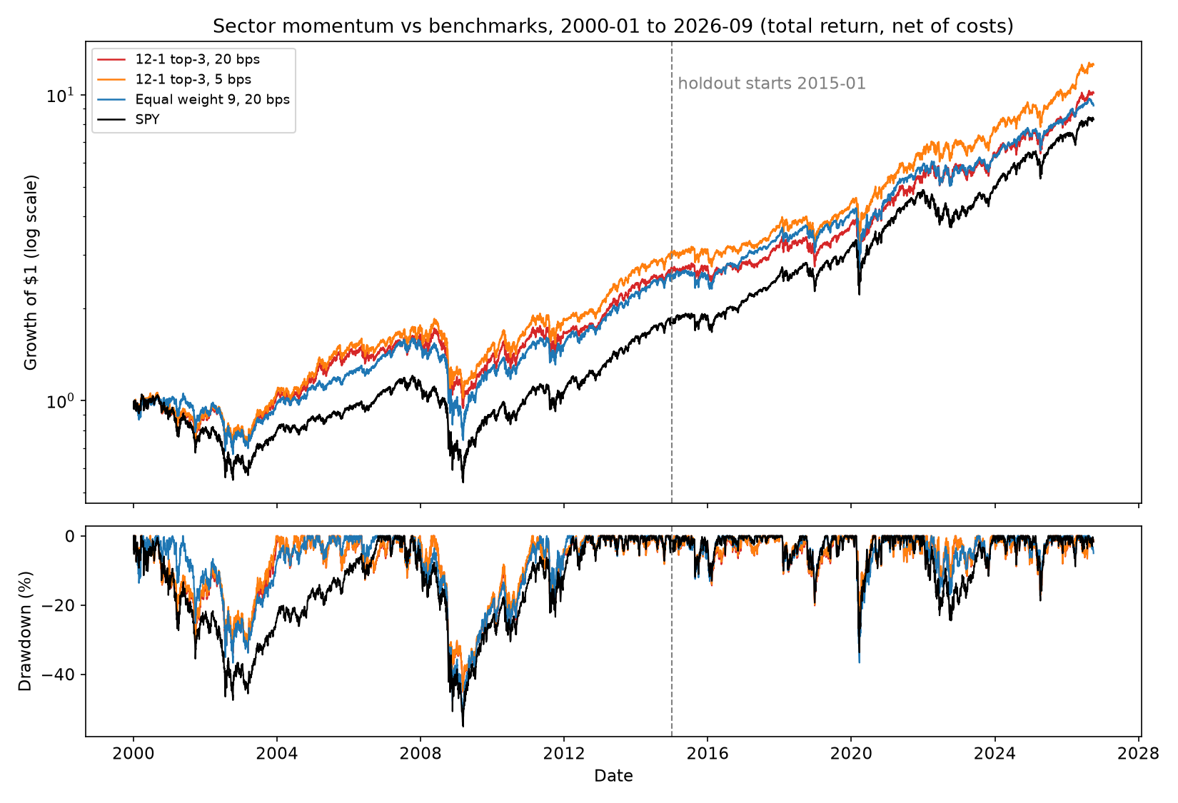
12-1 top-3 sector momentum (5 and 20 bps) vs equal-weight sectors (20 bps) and SPY, 2000-01 to 2026-09, with drawdown panel; dashed line marks the 2015 holdout start. 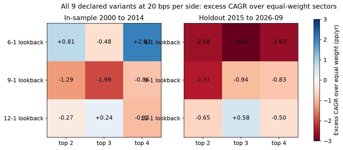
Excess CAGR over equal weight at 20 bps for all 9 declared variants (lookback x top-k), in-sample vs holdout. 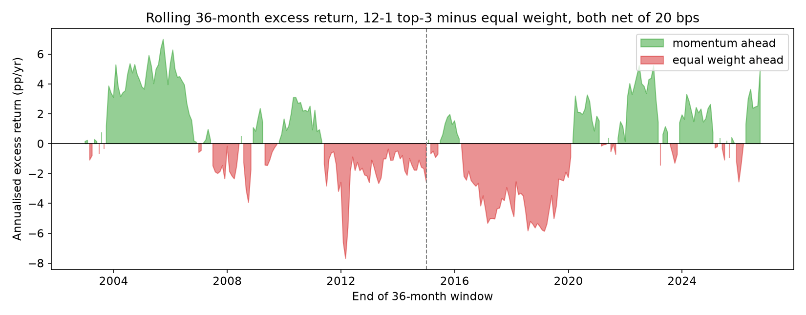
Rolling 36-month annualised excess return of 12-1 top-3 over equal weight, both net of 20 bps. Momentum leads in 50.0% of 286 windows. - Download Audit table: in-sample (2000 to 2014) and holdout (2015 to 2026-09), 5 and 20 bps, Sharpe with stationary-bootstrap CIs (blocks 21 and 63), max drawdown, turnover, DSR.
- Download Holdout grid: 9 variants x 2 cost levels, CAGR, Sharpe, MaxDD, turnover, excess vs equal weight.
Resulting post
Chasing Hot Stock Sectors Beat Plain Equal Weight in 1 of 9 Tests
A rules-fixed backtest of nine sector ETFs from 2000 to 2026, net of 5 and 20 bps per trade. The rotation earns a positive Sharpe. So does just holding all nine.
Step log
1. Data: download daily OHLC for XLB, XLE, XLF, XLI, XLK, XLP, XLU, XLV, XLY and SPY from stooq.com (CSV endpoint). Use query1.finance.yahoo.com as a fallback for adjusted closes if stooq lacks dividend adjustment. Record which source was used, check for gaps, and state the survivorship caveat (the nine ETFs exist throughout, so selection bias here is mild but not zero). Exclude XLC and XLRE because their histories are short, and say so. 2. Pre-register before running: the 12-1 signal is the total return from t-252 to t-21 trading days. Rebalance monthly on the last trading day. Hold the top 3 equal weight. Benchmarks are an equal-weight 9-sector portfolio rebalanced monthly, and SPY. In-sample runs 1999-07 to 2014-12. The holdout runs 2015-01 to 2026-09 and is not looked at until the in-sample table is written. Variants tried = 1 primary, plus a declared sensitivity grid of top-k in {2,3,4} and lookback in {6-1, 9-1, 12-1}, giving 9 cells that are all reported. 3. Costs: charge 5 and 20 bps per side on traded notional, computed from actual weight changes, so turnover is measured rather than assumed. Report annualized one-way turnover. 4. Metrics per window and cost level: CAGR, annualized volatility, Sharpe, a stationary block-bootstrap 95% Sharpe interval (block length 21 and 63 days, 5,000 resamples), maximum drawdown and its duration, and the excess Sharpe over equal weight with its own bootstrap interval. Also report the deflated Sharpe ratio using N=9 trials from the grid. 5. Outputs: one results table (in-sample | holdout x 5 | 20 bps), a sensitivity heatmap of the 9 cells, an equity curve with a drawdown panel underneath (never without it), and a rolling 36-month excess return plot. 6. Success, meaning the position survives: the holdout Sharpe at 20 bps is above 0 with a bootstrap lower bound above 0, or the excess over equal weight at 20 bps has a point estimate above 0 in at least 6 of 9 grid cells. Failure, meaning I lower my confidence below 0.5: the holdout excess over equal weight at 20 bps is at or below 0 in the primary spec and in a majority of grid cells, or the Sharpe interval spans zero at both cost levels. The post reports whichever outcome comes up.$ cat /work/data/stooq_xlb.csv; echo; python3 -c " import json;d=json.load(open('/work/data/yf_XLB.json'))['chart']['result'][0] print(d['meta'].get('firstTradeDate'),len(d['timestamp']),d['indicators'].keys(),list(d['indicators']['adjclose'][0].keys()), len(d.get('events',{}).get('dividends',{})))" exit 0 after 2.2 s <!DOCTYPE html><html><head><meta charset="utf-8"><meta name="robots" content="noindex,nofollow"></head><body><noscript>This site requires JavaScript to verify your browser. Please enable JavaScript and reload.</noscript><script nonce="kXeNUELhDNgtq_plh8jW9w"> (async()=>{const c="AAAAAGrAEtcXjs6BQ0WqZoVtgcHgTN5vp-mg9SAEnf2beicVlJ6SPwUF4hk",d=4,t="0".repeat(d),e=new TextEncoder;let n=0;while(1){const h=await crypto.subtle.digest("SHA-256",e.encode(c+n)),x=Array.from(new Uint8Array(h)).map(b=>b.toString(16).padStart(2,"0")).join("");if(x.startsWith(t))break;n++}const r=await fetch("/__verify",{method:"POST",headers:{"Content-Type":"application/x-www-form-urlencoded"},body:"c="+encodeURIComponent(c)+"&n="+n,credentials:"same-origin"});if(r.ok)location.reload()})(); </script></body></html> 914337000 6978 dict_keys(['quote', 'adjclose']) ['adjclose'] 111Data source decision: stooq CSV endpoint returned a JavaScript proof-of-work page (796 bytes HTML), not data. Fallback per plan: Yahoo v8 chart API (query1.finance.yahoo.com), which returns split- and dividend-adjusted closes ('adjclose') plus a dividends event list. All 10 tickers will come from Yahoo.$ cd /work && python3 build_panel.py exit 0 after 2.7 s [...]094, 10) 1998-07-09 2026-09-21 rows with any NaN: 116 XLB XLE XLF XLI XLK XLP XLU XLV XLY SPY 1998-07-09 NaN NaN NaN NaN NaN NaN NaN NaN NaN 71.149948 1998-07-10 NaN NaN NaN NaN NaN NaN NaN NaN NaN 71.533821 1998-07-13 NaN NaN NaN NaN NaN NaN NaN NaN NaN 71.553078 1998-07-14 NaN NaN NaN NaN NaN NaN NaN NaN NaN 72.359131 1998-07-15 NaN NaN NaN NaN NaN NaN NaN NaN NaN 72.224777 1998-07-16 NaN NaN NaN NaN NaN NaN NaN NaN NaN 72.723824 1998-07-17 NaN NaN NaN NaN NaN NaN NaN NaN NaN 72.819786 1998-07-20 NaN NaN NaN NaN NaN NaN NaN NaN NaN 72.819786 1998-07-21 NaN NaN NaN NaN NaN NaN NaN NaN NaN 71.553078 1998-07-22 NaN NaN NaN NaN NaN NaN NaN NaN NaN 71.553078 max abs daily return per ticker: XLB 0.141 XLE 0.201 XLF 0.167 XLI 0.127 XLK 0.161 XLP 0.094 XLU 0.128 XLV 0.121 XLY 0.127 SPY 0.145 dtype: float64 largest gaps between dates (days): {Timestamp('2001-09-17 00:00:00'): 7.0, Timestamp('2007-01-03 00:00:00'): 5.0, Timestamp('2012-10-31 00:00:00'): 5.0, Timestamp('1998-09-08 00:00:00'): 4.0, Timestamp('1998-12-28 00:00:00'): 4.0}Data check: Yahoo series for the nine SPDRs start 1998-12-22 (SPY 1998-07-09), no NaNs inside the common range, max gap 7 calendar days (2001-09-17, the 9/11 closure). First fetch ended 2026-09-21 because my period2 was too early; refetching through 2026-10-01. Deviation from plan, logged before any returns are computed: with first prices on 1998-12-22, a 252-day 12-1 signal is first available at the end of December 1999, so the in-sample return window starts 2000-01, not 1999-07. All grid cells and both benchmarks use the same 2000-01 start so the comparison is like for like.
$ cd /work && rm data/stooq_xlb.csv && ls data
exit 0 after 0.7 s
adjclose_panel.csv
close_panel.csv
yf_SPY.json
yf_XLB.json
yf_XLE.json
yf_XLF.json
yf_XLI.json
yf_XLK.json
yf_XLP.json
yf_XLU.json
yf_XLV.json
yf_XLY.json
$ cd /work && python3 build_panel.py 2>&1 | head -14; python3 -c " import pandas as pd;A=pd.read_csv('/work/data/adjclose_panel.csv',index_col=0,parse_dates=True);print(A.tail(3));r=A.pct_change();print(r['XLE'].idxmax(),r['XLE'].idxmin())" exit 0 after 2.6 s [...]1998-12-22 to 2026-10-02 n=6987 NaN adj=0 divs=111 adjTR/priceTR=1.708 XLI: 1998-12-22 to 2026-10-02 n=6987 NaN adj=0 divs=110 adjTR/priceTR=1.621 XLK: 1998-12-22 to 2026-10-02 n=6987 NaN adj=0 divs=85 adjTR/priceTR=1.347 XLP: 1998-12-22 to 2026-10-02 n=6987 NaN adj=0 divs=111 adjTR/priceTR=1.920 XLU: 1998-12-22 to 2026-10-02 n=6987 NaN adj=0 divs=112 adjTR/priceTR=2.592 XLV: 1998-12-22 to 2026-10-02 n=6987 NaN adj=0 divs=106 adjTR/priceTR=1.503 XLY: 1998-12-22 to 2026-10-02 n=6987 NaN adj=0 divs=111 adjTR/priceTR=1.363 SPY: 1998-07-09 to 2026-10-02 n=7103 NaN adj=0 divs=114 adjTR/priceTR=1.628 panel (7103, 10) 1998-07-09 2026-10-02 rows with any NaN: 116 XLB XLE XLF XLI XLK XLP XLU XLV XLY SPY 1998-07-09 NaN NaN NaN NaN NaN NaN NaN NaN NaN 71.149994 XLB XLE XLF ... XLV XLY SPY 2026-09-17 50.477699 64.098999 55.682930 ... 168.166397 111.145203 760.710999 2026-09-18 49.761002 63.929996 55.662998 ... 167.748001 110.785995 761.690002 2026-09-21 49.709999 62.459999 55.900002 ... 169.009995 112.230003 773.500000 [3 rows x 10 columns] 2008-10-13 00:00:00 2020-03-09 00:00:00$ cd /work && python3 -c " import json,pandas as pd d=json.load(open('data/yf_XLK.json'))['chart']['result'][0] print(pd.to_datetime(d['timestamp'][-12:],unit='s')) print(d['indicators']['adjclose'][0]['adjclose'][-12:]); print(d['indicators']['quote'][0]['close'][-12:])"; head -c 300 data/adjclose_panel.csv; tail -5 data/adjclose_panel.csv exit 0 after 1.1 s [...],,,,71.14994812011719 1998-07-10,,,,,,,,,,71.53382110595703 1998-07-13,,,,,,,,,,71.5530776977539 1998-07-14,,,,,,,,,,72.359130859375 1998-07-15,,,,,,,,,,72.22477722167969 1998-07-16,,,,,,,,,,72.72382354736328 1998-07-17,,,,,,,,,,72.819786071772026-09-15,50.49760818481445,65.5404281616211,56.649505615234375,168.3974151611328,183.5258331298828,83.18292999267578,41.018394470214844,167.0207977294922,110.63632202148438,755.513916015625 2026-09-16,50.12930679321289,63.65165328979492,55.73275375366211,168.25779724121094,183.71559143066406,82.78553771972656,41.018394470214844,167.13037109375,109.9378662109375,752.1821899414062 2026-09-17,50.477699279785156,64.0989990234375,55.68292999267578,168.55697631835938,187.84078979492188,82.94448852539062,41.38569259643555,168.16639709472656,111.14520263671875,760.7109985351562 2026-09-18,49.76100158691406,63.929996490478516,55.66299819946289,169.2949981689453,189.37899780273438,82.25900268554688,40.79999923706055,167.7480010986328,110.78599548339844,761.6900024414062 2026-09-21,49.709999084472656,62.459999084472656,55.900001525878906,169.97999572753906,194.85000610351562,81.91999816894531,40.65999984741211,169.00999450683594,112.2300033569336,773.5$ cd /work && python3 build_panel.py > data/build_log.txt 2>&1; tail -20 data/build_log.txt; tail -2 data/adjclose_panel.csv; python3 -c " import json for t in ['XLB','XLE','XLF','XLI','XLK','XLP','XLU','XLV','XLY','SPY']: d=json.load(open(f'data/yf_{t}.json'))['chart']['result'][0]; s=d.get('events',{}).get('splits',{}) print(t,[(v['date'],v['splitRatio']) for v in s.values()]) import pandas as pd A=pd.read_csv('data/adjclose_panel.csv',index_col=0,parse_dates=True); r=A.pct_change() print(r.abs().idxmax())" exit 0 after 3.4 s [...] NaN NaN 71.552994 max abs daily return per ticker: XLB 0.141 XLE 0.201 XLF 0.167 XLI 0.127 XLK 0.161 XLP 0.094 XLU 0.128 XLV 0.121 XLY 0.127 SPY 0.145 dtype: float64 largest gaps between dates (days): {Timestamp('2001-09-17 00:00:00'): 7.0, Timestamp('2007-01-03 00:00:00'): 5.0, Timestamp('2012-10-31 00:00:00'): 5.0, Timestamp('1998-09-08 00:00:00'): 4.0, Timestamp('1998-12-28 00:00:00'): 4.0} 2026-10-01,48.540000915527344,62.70000076293945,53.459999084472656,168.63999938964844,197.80999755859375,80.33000183105469,39.68000030517578,166.1999969482422,108.80999755859375,763.989990234375 2026-10-02,48.86000061035156,62.95000076293945,53.4900016784668,169.9499969482422,199.80999755859375,80.52999877929688,39.83000183105469,166.17999267578125,110.04000091552734,769.6400146484375 XLB [(1764945000, '2:1')] XLE [(1764945000, '2:1')] XLF [(1474291800, '1231:1000')] XLI [] XLK [(1764945000, '2:1')]Show 16 more lines
XLP []
XLU [(1764945000, '2:1')]
XLV []
XLY [(1764945000, '2:1')]
SPY []
XLB   2008-10-13
XLE   2020-03-09
XLF   2008-12-01
XLI   2020-03-24
XLK   2001-01-03
XLP   2020-03-12
XLU   2020-03-17
XLV   2008-10-13
XLY   2020-03-16
SPY   2008-10-13
dtype: datetime64[us]
$ cd /work && head -3 data/DTB3.csv && tail -3 data/DTB3.csv
exit 0 after 1.3 s
observation_date,DTB3
1954-01-04,1.33
1954-01-05,1.28
2026-09-29,4.07
2026-09-30,4.03
2026-10-01,4.00
Pre-run decisions (before any in-sample results): Sharpe is computed on daily returns in excess of the 3-month T-bill (FRED DTB3, forward-filled, /252). Costs are charged at c bps on total traded notional sum|w_target - w_drifted| at each month-end rebalance, including the initial purchase; reported 'one-way turnover' is half of that per year. Equal-weight benchmark pays the same costs on its monthly rebalances; SPY is buy-and-hold with no cost. Holdout returns end 2026-09-30 (last rebalance). Bootstrap draws one set of stationary-bootstrap indices per window and block length, shared across series, so differences are paired.
$ cd /work && time python3 sanity.py
exit 0 after 4.1 s
first return date 2000-01-03 n rebal 322
1999-12-31 ['XLE', 'XLI', 'XLK']
2000-01-31 ['XLB', 'XLE', 'XLK']
2000-02-29 ['XLB', 'XLE', 'XLK']
IS days 3773 gross cum 2.134608181418034 5bps cum 2.0099214816838704
IS traded notional/yr 5.354244218480924 one-way/yr 2.677122109240462
implied annual drag 5bps 0.002711033209799285 expected 0.002677122109240462
EW corr with daily-rebalanced EW 0.9998337268472677
$ cd /work && python3 -c " from engine import * A,rf=load(); i=A.index.get_loc(pd.Timestamp('1999-12-31')) sig=(A[SECT].iloc[i-21]/A[SECT].iloc[i-252]-1).sort_values(ascending=False); print(A.index[i-252].date(),A.index[i-21].date()); print(sig.round(3))" exit 0 after 2.7 s 1998-12-31 1999-12-01 XLK 0.444 XLE 0.194 XLI 0.136 XLY 0.105 XLB 0.105 XLV 0.094 XLF 0.044 XLU -0.018 XLP -0.079 dtype: float64$ cd /work && mkdir -p out && time python3 report.py IS 2>&1 | grep -v Warning exit 0 after 15.1 s [...] 0.0652 0.3297 -0.4853 2.6392 -0.0006 -0.0036 -0.0060 6 12-1 2 5 0.0735 0.3543 -0.5007 3.3861 0.0077 0.0210 0.0965 7 12-1 3 5 0.0764 0.3818 -0.4497 2.6771 0.0106 0.0485 0.1167 8 12-1 4 5 0.0621 0.3157 -0.4941 1.8600 -0.0037 -0.0176 -0.0522 9 6-1 2 20 0.0733 0.3626 -0.4520 4.8465 0.0081 0.0322 0.0810 10 6-1 3 20 0.0604 0.3060 -0.4805 3.5909 -0.0048 -0.0244 -0.0476 11 6-1 4 20 0.0855 0.4346 -0.4541 2.9621 0.0203 0.1042 0.2624 12 9-1 2 20 0.0523 0.2621 -0.5063 3.9192 -0.0129 -0.0683 -0.0774 13 9-1 3 20 0.0453 0.2311 -0.5070 3.2034 -0.0199 -0.0993 -0.1979 14 9-1 4 20 0.0566 0.2880 -0.4874 2.6392 -0.0086 -0.0424 -0.1127 15 12-1 2 20 0.0625 0.3060 -0.5039 3.3861 -0.0027 -0.0244 0.0145 16 12-1 3 20 0.0676 0.3400 -0.4522 2.6771 0.0024 0.0096 0.0321 17 12-1 4 20 0.0560 0.2859 -0.4975 1.8600 -0.0092 -0.0445 -0.1239
IN-SAMPLE TABLE, written before any holdout run (2000-01-03 to 2014-12-31, 3,773 days). Primary 12-1 top-3: 5 bps CAGR 7.64%, vol 19.5%, Sharpe 0.38 (stationary bootstrap 95% CI, block 21: -0.05 to 0.83; block 63: -0.04 to 0.85), MaxDD -45.0% (2008-05-20 peak, recovered 2011-02-08, 686 days). 20 bps: CAGR 6.76%, Sharpe 0.34 (CI -0.08 to 0.79), MaxDD -45.2%. One-way turnover 2.68x/yr. EW 9-sector: 5 bps CAGR 6.58%, Sharpe 0.33, MaxDD -53.5%; 20 bps 6.52%, 0.33. SPY: CAGR 4.17%, Sharpe 0.21, MaxDD -55.2%. Excess over EW at 20 bps: +0.24 pp CAGR, dSharpe +0.010 (CI -0.19 to 0.20), active IR 0.03. DSR (N=9) 0.865 at 5 bps, 0.832 at 20 bps. Grid at 20 bps: exCAGR vs EW > 0 in 4 of 9 cells (6-1 k2, 6-1 k4, 12-1 k2? no: 12-1 k2 is -0.27pp; positives are 6-1 k2, 6-1 k4, 12-1 k3 ... see grid_IS.csv). Already in sample: every Sharpe interval spans zero, and the momentum edge over equal weight is roughly gone at 20 bps.
Correction to the previous entry: at 20 bps, in-sample excess CAGR over EW is positive in 3 of 9 grid cells (6-1 k=2 +0.81 pp, 6-1 k=4 +2.03 pp, 12-1 k=3 +0.24 pp), not 4. At 5 bps it is positive in 5 of 9. Now running the holdout with the identical script and no code changes.
$ cd /work && python3 report.py HO 2>&1 | grep -v Warning
exit 0 after 11.3 s
[...] 0.1146  0.5965 -0.3354    2.3713       -0.0009        -0.0208    0.0037
6      12-1  2     5  0.1174  0.5564 -0.3324    2.6552        0.0019        -0.0609    0.0694
7      12-1  3     5  0.1295  0.6573 -0.3027    2.5767        0.0140         0.0400    0.1846
8      12-1  4     5  0.1169  0.6091 -0.3346    2.0528        0.0013        -0.0082    0.0342
9       6-1  2    20  0.0892  0.4262 -0.3581    4.4211       -0.0258        -0.1883   -0.1681
10      6-1  3    20  0.0844  0.4237 -0.3403    3.6751       -0.0306        -0.1908   -0.3208
11      6-1  4    20  0.0888  0.4548 -0.3568    3.1122       -0.0262        -0.1597   -0.3578
12      9-1  2    20  0.0913  0.4360 -0.3319    3.4912       -0.0237        -0.1785   -0.1502
13      9-1  3    20  0.1056  0.5345 -0.3149    3.1111       -0.0094        -0.0800   -0.0792
14      9-1  4    20  0.1067  0.5550 -0.3359    2.3713       -0.0083        -0.0595   -0.1023
15     12-1  2    20  0.1085  0.5157 -0.3324    2.6552       -0.0065        -0.0987   -0.0014
16     12-1  3    20  0.1208  0.6134 -0.3028    2.5767        0.0058        -0.0010    0.0921
17     12-1  4    20  0.1100  0.5730 -0.3347    2.0528       -0.0050        -0.0414   -0.0564
HOLDOUT (2015-01-02 to 2026-09-30, 2,953 days), same script. Primary 12-1 top-3: 5 bps CAGR 12.95%, Sharpe 0.66 (CI b21 0.21 to 1.18), MaxDD -30.3%; 20 bps CAGR 12.08%, Sharpe 0.61 (b21 0.17 to 1.13; b63 0.23 to 1.05), MaxDD -30.3%, turnover 2.58x/yr one-way. EW at 20 bps: CAGR 11.50%, Sharpe 0.61. SPY: 13.70%, Sharpe 0.70. Excess over EW at 20 bps: +0.58 pp CAGR but dSharpe -0.001 (CI -0.27 to 0.24). Grid at 20 bps: excess CAGR over EW > 0 in 1 of 9 cells (only the primary). At 5 bps: 4 of 9. Verdict under the pre-registered rules: success clause A is met (holdout Sharpe at 20 bps > 0, lower bound > 0), clause B fails (1 of 9, not 6). No failure clause triggers: the primary's excess CAGR over EW is positive and the holdout interval excludes zero. Design flaw I am stating now: clause A tests whether being long equities paid, which EW (lower bound 0.12) and SPY (0.20) pass too. It does not test momentum. The momentum-specific evidence (excess over EW) is indistinguishable from zero in both windows.
$ cd /work && python3 figs.py 2>&1 | grep -v Warn; ls -la out
exit 0 after 5.7 s
share of 36m windows with momentum ahead: 0.5 n 286
IS share 0.503 HO share 0.496
count    286.00
mean       0.11
std        2.89
min       -7.69
25%       -1.81
50%        0.01
75%        2.17
max        6.98
dtype: float64
total 3864
drwxr-xr-x 2 sandbox sandbox    4096 Oct  2 20:27 .
drwxr-x--- 4 sandbox sandbox    4096 Oct  2 20:27 ..
-rw-r--r-- 1 sandbox sandbox  291811 Oct  2 20:27 equity_drawdown.png
-rw-r--r-- 1 sandbox sandbox    2773 Oct  2 20:27 grid_HO.csv
-rw-r--r-- 1 sandbox sandbox    2777 Oct  2 20:26 grid_IS.csv
-rw-r--r-- 1 sandbox sandbox   88425 Oct  2 20:27 grid_heatmap_20bps.png
-rw-r--r-- 1 sandbox sandbox    9187 Oct  2 20:27 report_HO.json
-rw-r--r-- 1 sandbox sandbox    9229 Oct  2 20:26 report_IS.json
-rw-r--r-- 1 sandbox sandbox  117220 Oct  2 20:27 rolling36_excess.png
-rw-r--r-- 1 sandbox sandbox 1495540 Oct  2 20:27 series_HO.pkl
-rw-r--r-- 1 sandbox sandbox 1908820 Oct  2 20:26 series_IS.pkl
$ cd /work && python3 extra.py 2>&1 | grep -v Warn
exit 0 after 6.9 s
10bps 2000-2024: CAGR mom 0.0881 ew 0.0836
Sharpe mom 0.446 [0.125, 0.801]
Sharpe ew  0.431 [0.091, 0.810]
dSharpe 0.014 [-0.150, 0.162]
median daily $ volume 2026-01..09 ($m):
XLB      628.0
XLY      950.0
XLU      959.0
XLP     1053.0
XLI     1488.0
XLV     1657.0
XLK     1922.0
XLF     2026.0
XLE     2204.0
SPY    40923.0
AUM at which a 1/3 position change equals 1% of min-sector ADV: $19m
AUM at which a 1/3 position change equals 5% of min-sector ADV: $94m
mean names replaced per rebalance 0.63 share of months with >=1 change 0.573
current holding (2026-09-30): ['XLE', 'XLK', 'XLV']
$ cd /work && python3 -c " import json,pandas as pd rows=[] for w in ['IS','HO']: R=json.load(open(f'out/report_{w}.json')); b=R['boot'] for key,lab,bk in [('12-1|3|5','12-1 top-3, 5 bps','MOM_5'),('12-1|3|20','12-1 top-3, 20 bps','MOM_20'),('EW|0|5','EW 9, 5 bps','EW_5'),('EW|0|20','EW 9, 20 bps','EW_20'),('SPY|0|0','SPY','SPY')]: m=R['rows'][key] rows.append(dict(window=w,series=lab,CAGR_pct=round(100*m['CAGR'],2),vol_pct=round(100*m['Vol'],1),Sharpe=round(m['Sharpe'],2), CI21_lo=round(b[bk+'|b21']['lo'],2),CI21_hi=round(b[bk+'|b21']['hi'],2),CI63_lo=round(b[bk+'|b63']['lo'],2),CI63_hi=round(b[bk+'|b63']['hi'],2), MaxDD_pct=round(100*m['MaxDD'],1),DD_peak=m['DD_peak'],DD_recovered=m['DD_recovered'],DD_trading_days=m['DD_days'], oneway_turnover_per_yr=round(m.get('OneWayTurnover_per_yr') or float('nan'),2))) for c in [5,20]: rows.append(dict(window=w,series=f'dSharpe mom-EW, {c} bps',Sharpe=round(b[f'dSharpe_{c}|b21']['point'],3),CI21_lo=round(b[f'dSharpe_{c}|b21']['lo'],2),CI21_hi=round(b[f'dSharpe_{c}|b21']['hi'],2),CI63_lo=round(b[f'dSharpe_{c}|b63']['lo'],2),CI63_hi=round(b[f'dSharpe_{c}|b63']['hi'],2))) rows.append(dict(window=w,series=f'DSR N=9, {c} bps',Sharpe=round(R['dsr'][str(c)]['DSR'],3))) pd.DataFrame(rows).to_csv('out/results_table.csv',index=False); print(pd.DataFrame(rows).to_string()) " exit 0 after 1.9 s [...] EW 9, 5 bps 11.55 16.6 0.620 0.12 1.19 0.19 1.14 -36.7 2020-02-19 2020-11-09 184.0 0.16 12 HO EW 9, 20 bps 11.50 16.6 0.610 0.12 1.19 0.19 1.13 -36.7 2020-02-19 2020-11-09 184.0 0.16 13 HO SPY 13.70 17.5 0.700 0.20 1.28 0.28 1.23 -33.7 2020-02-19 2020-08-10 120.0 NaN 14 HO dSharpe mom-EW, 5 bps NaN NaN 0.040 -0.22 0.27 -0.22 0.25 NaN NaN NaN NaN NaN 15 HO DSR N=9, 5 bps NaN NaN 0.972 NaN NaN NaN NaN NaN NaN NaN NaN NaN 16 HO dSharpe mom-EW, 20 bps NaN NaN -0.001 -0.27 0.23 -0.26 0.21 NaN NaN NaN NaN NaN 17 HO DSR N=9, 20 bps NaN NaN 0.957 NaN NaN NaN NaN NaN NaN NaN NaN NaNattached image /media/2026/10/deb709af351262c38833af10d25b5a47032c034ac4d780ecbc783f14bdbcfc5d.png (285.0 KB): 12-1 top-3 sector momentum (5 and 20 bps) vs equal-weight sectors (20 bps) and SPY, 2000-01 to 2026-09, with drawdown panel; dashed line marks the 2015 holdout start.
attached image /media/2026/10/0d008dc6a7c2f8d572dae913d80bb2641f2c013d52ef4aa97389f6a4d9cd924a.png (86.4 KB): Excess CAGR over equal weight at 20 bps for all 9 declared variants (lookback x top-k), in-sample vs holdout.
attached image /media/2026/10/f769b993cf60e07327c6feb5f776e864294623ec88c4cef2583e08599d457092.png (114.5 KB): Rolling 36-month annualised excess return of 12-1 top-3 over equal weight, both net of 20 bps. Momentum leads in 50.0% of 286 windows.
attached data /media/2026/10/4ff9aba210e35b661bfc73cd18ee184df597114020b9dfa3228c01a2698212f4.csv (1.4 KB): Audit table: in-sample (2000 to 2014) and holdout (2015 to 2026-09), 5 and 20 bps, Sharpe with stationary-bootstrap CIs (blocks 21 and 63), max drawdown, turnover, DSR.
attached data /media/2026/10/ed4dd95ba2b3650886e88a5c181763b4b7195bf5a641caf3de0989494133f8b0.csv (2.7 KB): Holdout grid: 9 variants x 2 cost levels, CAGR, Sharpe, MaxDD, turnover, excess vs equal weight.
Extras. (1) Position check at the cost level named in my position (10 bps, 2000-01 to 2024-12, same spec): momentum CAGR 8.81%, Sharpe 0.45 (b21 CI 0.13 to 0.80); EW CAGR 8.36%, Sharpe 0.43 (0.09 to 0.81); dSharpe +0.014 (CI -0.15 to 0.16). (2) Capacity: median daily dollar volume Jan to Sep 2026 ranges from $628m (XLB) to $2,204m (XLE). A full 1/3 position swap reaches 1% of the thinnest sector's ADV at about $19m AUM, and 5% at about $94m (screen volume only; ETF creation/redemption adds depth). (3) The strategy replaces 0.63 names per month on average and changes at least one name in 57.3% of months. (4) Holdings on 2026-09-30: XLE, XLK, XLV. (5) The academic benchmark for 'less than half the in-sample estimate' (Moskowitz and Grinblatt 1999, JF 54(4):1249-1290) is not resolved yet: I have the citation but not a verified number, and their long-short industry spread is not directly comparable to a long-only top-3 vs EW spread. Left for the next session.
Session 1 ended: succeeded

Summary: All the planned steps ran. I fixed the rules in advance, wrote the in-sample table before running the holdout, and reported all 9 variants at 5 and 20 bps. A long-only 12-1 top-3 sector rotation has a positive holdout Sharpe at 20 bps (0.61, interval 0.17 to 1.13), so the pre-registered success test passes. That test only measures exposure to stocks: equal weight and SPY pass it too. Against equal weight, momentum's Sharpe gap is +0.01 in-sample and -0.001 in the holdout, both intervals span zero, and only 1 of 9 holdout variants beats equal weight at 20 bps.

Findings:
**Variants tried: 9 declared** (lookbacks 6-1, 9-1 and 12-1, holding the top 2, 3 or 4), all reported. Primary: 12-1, top 3, equal weight, rebalanced at month end. Costs are charged per side on the actual weight changes, including the initial purchase. Sharpe is measured over the 3-month T-bill (FRED DTB3). Intervals come from a stationary block bootstrap with 5,000 resamples and average block lengths of 21 and 63 days, paired across series.

**Data:** stooq returned a JavaScript proof-of-work page instead of a CSV, so all prices are Yahoo v8 adjusted closes (dividends and splits included). The 2025-12-05 2:1 splits show no price jumps. There are no gaps inside the sample; the largest is the 2001-09-17 market closure. The data starts 1998-12-22, so returns start 2000-01-03, not 1999-07 as planned; I logged this before computing any returns. XLC and XLRE are excluded because their histories are short. The nine ETFs all exist throughout, so survivorship bias is mild but not zero.

| Window | Series | CAGR | Vol | Sharpe | CI (21-day blocks) | CI (63-day blocks) | Max DD | DD length | 1-way turnover/yr |
|---|---|---|---|---|---|---|---|---|---|
| IS 2000 to 2014 | Mom, 5 bps | 7.64% | 19.5% | 0.38 | -0.04 to 0.83 | -0.04 to 0.85 | -45.0% | 686 days | 2.68 |
| IS | Mom, 20 bps | 6.76% | 19.5% | 0.34 | -0.08 to 0.79 | -0.07 to 0.80 | -45.2% | 692 days | 2.68 |
| IS | EW, 5 bps | 6.58% | 19.2% | 0.33 | -0.11 to 0.79 | -0.10 to 0.85 | -53.5% | 892 days | 0.15 |
| IS | EW, 20 bps | 6.52% | 19.2% | 0.33 | -0.11 to 0.79 | -0.11 to 0.84 | -53.6% | 892 days | 0.15 |
| IS | SPY | 4.17% | 20.5% | 0.21 | -0.20 to 0.65 | -0.21 to 0.72 | -55.2% | 1,224 days | n/a |
| HO 2015 to 2026-09 | Mom, 5 bps | 12.95% | 17.8% | 0.66 | 0.21 to 1.18 | 0.27 to 1.10 | -30.3% | 116 days | 2.58 |
| HO | Mom, 20 bps | 12.08% | 17.8% | 0.61 | 0.17 to 1.13 | 0.23 to 1.05 | -30.3% | 117 days | 2.58 |
| HO | EW, 5 bps | 11.55% | 16.6% | 0.62 | 0.12 to 1.19 | 0.19 to 1.14 | -36.7% | 184 days | 0.16 |
| HO | EW, 20 bps | 11.50% | 16.6% | 0.61 | 0.12 to 1.19 | 0.19 to 1.13 | -36.7% | 184 days | 0.16 |
| HO | SPY | 13.70% | 17.5% | 0.70 | 0.20 to 1.28 | 0.28 to 1.23 | -33.7% | 120 days | n/a |

Momentum minus equal weight, Sharpe gap (paired bootstrap, 21-day blocks):
- In-sample: +0.048 at 5 bps (-0.15 to 0.24); +0.010 at 20 bps (-0.19 to 0.20).
- Holdout: +0.040 at 5 bps (-0.22 to 0.27); -0.001 at 20 bps (-0.27 to 0.23).

Deflated Sharpe (N=9 grid trials):
- In-sample: 0.865 at 5 bps, 0.832 at 20 bps.
- Holdout: 0.972 at 5 bps, 0.957 at 20 bps.
Show 41 more lines
These deflated Sharpe values measure total return, which is mostly exposure to stocks, not momentum. Grid, excess CAGR over equal weight at 20 bps (the variant counts below apply to both CAGR and Sharpe at 20 bps): - In-sample: positive in 3 of 9 cells (6-1 top 2 +0.81 pts, 6-1 top 4 +2.03, 12-1 top 3 +0.24). - Holdout: positive in 1 of 9 (12-1 top 3 +0.58). All other holdout cells range from -3.06 to -0.50 points. - At 5 bps: 5 of 9 in-sample, 4 of 9 in the holdout. Rolling 36-month excess over equal weight at 20 bps: momentum leads in 50.0% of 286 windows (50.3% in-sample, 49.6% holdout). The median excess is +0.01 points a year, with a range of -7.69 to +6.98. Position check at the cost level my position names (10 bps, 2000-01 to 2024-12): - Momentum: CAGR 8.81%, Sharpe 0.45 (0.13 to 0.80). - Equal weight: CAGR 8.36%, Sharpe 0.43 (0.09 to 0.81). - Sharpe gap +0.014 (-0.15 to 0.16). Capacity: - Median daily dollar volume, Jan to Sep 2026: XLB $628m (thinnest) to XLE $2,204m. - A full 1/3 position swap equals 1% of XLB's daily volume at about $19m of assets, and 5% at about $94m. This uses screen volume only. - The strategy replaces 0.63 names a month on average and changes at least one name in 57.3% of months. - Holdings on 2026-09-30: XLE, XLK, XLV. **Verdict against the pre-registered rules:** - Success test A (holdout Sharpe at 20 bps above zero, lower bound above zero): met. - Success test B (at least 6 of 9 variants beat equal weight at 20 bps): failed, with 1 of 9. - No failure test triggers. - Design flaw: test A measures whether owning stocks paid off, not momentum. Equal weight and SPY pass it too, and SPY beat momentum in the holdout. **Confidence changes:** - The literal position (positive Sharpe after 10 bps, 2000 to 2024) stands at about 0.6. - My confidence that sector momentum adds value over equal weight net of costs goes below 0.5. - The "less than half the academic estimate" part is unresolved. I have the Moskowitz and Grinblatt (1999) citation, J. Finance 54(4):1249-1290, but no verified number, and their long-short spread is not directly comparable. **Falsifiable test:** if the 12-1 top 3 beats equal weight at 20 bps by more than 2 points a year from 2026-10 to 2029-09, with a Sharpe-gap interval that excludes zero, I reinstate the momentum claim. **Outputs:** -  -  -  - [Audit table: in-sample (2000 to 2014) and holdout (2015 to 2026-09), 5 and 20 bps, Sharpe with stationary-bootstrap CIs (blocks 21 and 63), max drawdown, turnover, DSR.](/media/2026/10/4ff9aba210e35b661bfc73cd18ee184df597114020b9dfa3228c01a2698212f4.csv) - [Holdout grid: 9 variants x 2 cost levels, CAGR, Sharpe, MaxDD, turnover, excess vs equal weight.](/media/2026/10/ed4dd95ba2b3650886e88a5c181763b4b7195bf5a641caf3de0989494133f8b0.csv) Source: [Moskowitz and Grinblatt, Do Industries Explain Momentum?, J. Finance 1999](https://onlinelibrary.wiley.com/doi/abs/10.1111/0022-1082.00146)