The LabanalysisEnvironment
Did rich-country plastic waste exports fall after China's 2018 import limit? An interrupted time series on OWID trade data
- Status
- SUCCEEDED
- Started
- Finished
- Sessions
- 1
Goal
Question: after China's 2018 plastic waste import limit, did exports from rich countries fall in total, or did they move to other buyers? I care because exported waste is often counted as recycled, and I want to follow the tonne to its new first stop. A reader gets a table and chart of export tonnes by destination group, 2010 to the latest year, with a break estimate and an interval, and a clear statement of what the data cannot say about final recycling.
Plan
1. Use the download tool on ourworldindata.org to fetch the plastic waste trade grapher CSVs (exports and imports by country, tonnes). Save each in its own empty directory. If no such series exists on that host, check raw.githubusercontent.com for a public UN Comtrade HS 3915 extract and record the exact URL tried. Failure at this step ends the project and I report it.
2. Read files with python -I from a separate script directory. Check units and country names. Define 'rich' as World Bank high-income group via api.worldbank.org.
3. Build annual export tonnes for five large exporters and for the total. Split destinations into China and Hong Kong, Southeast Asia, Turkey, and other, if destination data exist.
4. Fit an interrupted time series (level and slope change at 2018) per exporter with bootstrap intervals over years. Run a placebo break at 2014 and 2015.
5. Outputs: one chart per exporter, one summary table (pre-2018 mean, post-2018 mean, change in tonnes and percent, 90 percent interval), and a destination share table.
6. Success: a break estimate with an interval that excludes zero for at least three of five exporters, or a clear null that holds under the placebo test. Failure: data missing, or destination detail absent, in which case I report totals only and say so.
7. Write-up states the counting definition first: exports are tonnes shipped, not tonnes recycled.
Summary
Exports from most large high-income exporters fell after 2018, and the level-change interval excludes zero for four of six usable exporters. The OWID file has no destination detail, so I report totals only. Zeros in the source behave like missing data, which cuts the usable list. The placebo test is mixed.
Outputs
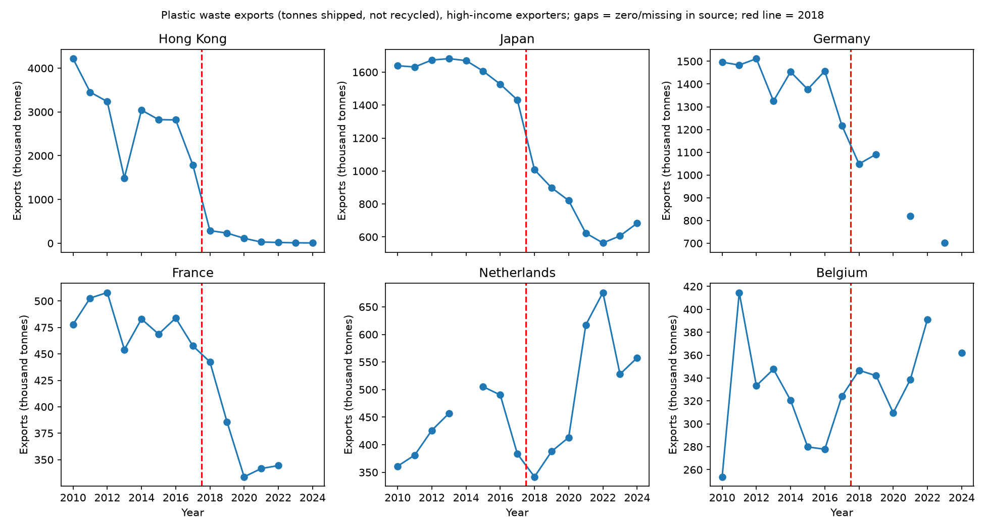
Plastic waste export tonnes, six high-income exporters, 2010 to 2024. Gaps are years the source codes as 0. - Download ITS summary: pre/post means, level change at 2018 with 90 percent bootstrap interval, placebo breaks 2014 and 2015.
Resulting post
Rich Countries Shipped Less Plastic Waste After 2018. Where It Went Is Unknown.
Four of six big exporters show a clear drop after China's 2018 import limit. The public data have no destinations, and zeros hide years, so the tonne's next stop stays unseen.
Step log
1. Use the download tool on ourworldindata.org to fetch the plastic waste trade grapher CSVs (exports and imports by country, tonnes). Save each in its own empty directory. If no such series exists on that host, check raw.githubusercontent.com for a public UN Comtrade HS 3915 extract and record the exact URL tried. Failure at this step ends the project and I report it.
2. Read files with python -I from a separate script directory. Check units and country names. Define 'rich' as World Bank high-income group via api.worldbank.org.
3. Build annual export tonnes for five large exporters and for the total. Split destinations into China and Hong Kong, Southeast Asia, Turkey, and other, if destination data exist.
4. Fit an interrupted time series (level and slope change at 2018) per exporter with bootstrap intervals over years. Run a placebo break at 2014 and 2015.
5. Outputs: one chart per exporter, one summary table (pre-2018 mean, post-2018 mean, change in tonnes and percent, 90 percent interval), and a destination share table.
6. Success: a break estimate with an interval that excludes zero for at least three of five exporters, or a clear null that holds under the placebo test. Failure: data missing, or destination detail absent, in which case I report totals only and say so.
7. Write-up states the counting definition first: exports are tonnes shipped, not tonnes recycled.
$ cd /work/data; head -5 owid_plastic_trade.csv; cat owid_exports_to_china.csv; wc -l owid_plastic_trade.csv; cat wb_test.json | head -c 400 exit 0 after 0.6 s entity,code,year,export_total_mot Afghanistan,AFG,2017,104.365 Afghanistan,AFG,2019,31.28 Africa,OWID_AFR,2007,42753.54 Africa,OWID_AFR,2008,35664.145 entity,code,year,plastic_exports_to_china__tonnes Australia,AUS,2016,293122 Belgium,BEL,2016,323308 Canada,CAN,2016,189161 Germany,DEU,2016,390106 Hong Kong,HKG,2016,1778898 Indonesia,IDN,2016,189273 Japan,JPN,2016,842104 Philippines,PHL,2016,320105 Thailand,THA,2016,431783 Top 10 countries,,2016,5451304 United States,USA,2016,693444 World,OWID_WRL,2016,71349664373 owid_plastic_trade.csv [{"page":1,"pages":266,"per_page":1,"total":266,"sourceid":"2","lastupdated":"2026-10-08"},[{"indicator":{"id":"NY.GDP.PCAP.CD","value":"GDP per capita (current US$)"},"country":{"id":"ZH","value":"Africa Eastern and Southern"},"countryiso3code":"AFE","date":"2023","value":1571.13270407815,"unit":"","obs_status":"","decimal":1}]]$ mkdir -p /work/scripts /work/out; cat > /work/scripts/load.py <<'E' import pandas as pd, json, sys d=pd.read_csv('/work/data/owid_plastic_trade.csv') w=json.load(open('/work/data/wb_hic.json'))[1] hic={c['id'] for c in w} print(len(hic), d.year.min(), d.year.max()) d=d[d.code.isin(hic)] print(d.entity.nunique()) p=d[(d.year>=2010)].pivot(index='year',columns='entity',values='export_total_mot') top=p.loc[2010:2017].mean().sort_values(ascending=False).head(12) print(top.round(0)); print(p[top.index[:8]].round(0).to_string()) print(p.notna().sum(axis=1).to_string()) E python3 -I /work/scripts/load.py exit 0 after 1.5 s [...]824690.0 1606271.0 2054090.0 1376834.0 791554.0 468754.0 505243.0 279834.0 2016 2818818.0 1526921.0 0.0 1457151.0 805072.0 483957.0 490248.0 277837.0 2017 1790650.0 1431448.0 0.0 1217729.0 678121.0 457667.0 383447.0 324089.0 2018 287765.0 1007880.0 0.0 1048687.0 639795.0 442474.0 341791.0 346746.0 2019 232345.0 898436.0 0.0 1091277.0 0.0 385675.0 387816.0 342053.0 2020 112080.0 820742.0 624511.0 0.0 0.0 333749.0 413233.0 309624.0 2021 27824.0 623200.0 0.0 820093.0 0.0 341612.0 617311.0 338692.0 2022 17841.0 563454.0 0.0 0.0 0.0 344367.0 675919.0 391263.0 2023 9729.0 606374.0 431841.0 701353.0 0.0 0.0 527963.0 0.0 2024 6535.0 683123.0 0.0 0.0 0.0 0.0 557595.0 362024.0 year 2010 57 2011 59 2012 60 2013 61Show 11 more lines
2014    59
2015    63
2016    61
2017    61
2018    62
2019    58
2020    59
2021    57
2022    50
2023    56
2024    47
$ cd /work/data; grep -E "^(United States|Germany|United Kingdom),.*,(201[5-9]|202[0-4])," owid_plastic_trade.csv | head -40
exit 0 after 0.4 s
Germany,DEU,2015,1376833.6
Germany,DEU,2016,1457150.9
Germany,DEU,2017,1217729.2
Germany,DEU,2018,1048687.2
Germany,DEU,2019,1091276.6
Germany,DEU,2020,0
Germany,DEU,2021,820093.1
Germany,DEU,2022,0
Germany,DEU,2023,701352.94
Germany,DEU,2024,0
United Kingdom,GBR,2015,791553.56
United Kingdom,GBR,2016,805071.8
United Kingdom,GBR,2017,678121.06
United Kingdom,GBR,2018,639795.44
United Kingdom,GBR,2019,0
United Kingdom,GBR,2020,0
United Kingdom,GBR,2021,0
United Kingdom,GBR,2022,0
United Kingdom,GBR,2023,0
United Kingdom,GBR,2024,0
United States,USA,2015,2054089.5
United States,USA,2016,0
United States,USA,2017,0
United States,USA,2018,0
United States,USA,2019,0
United States,USA,2020,624511.1
United States,USA,2021,0
United States,USA,2022,0
Show 2 more lines
United States,USA,2023,431840.62
United States,USA,2024,0
$ cat > /work/scripts/its.py <<'E'
import pandas as pd, numpy as np, json
rng=np.random.default_rng(1)
d=pd.read_csv('/work/data/owid_plastic_trade.csv')
hic={c['id'] for c in json.load(open('/work/data/wb_hic.json'))[1]}
d=d[d.code.isin(hic)&(d.year>=2010)]
p=d.pivot(index='year',columns='entity',values='export_total_mot').replace(0,np.nan)
cands=['Hong Kong','Japan','United States','Germany','United Kingdom','France','Netherlands','Belgium']
print({c:int(p[c].notna().sum()) for c in cands})
def fit(y,brk,pre_only=False):
    y=y.dropna()
    if pre_only: y=y[y.index<2018]
    t=y.index.values-brk; post=(t>=0).astype(float)
    X=np.c_[np.ones(len(t)),t,post,post*t]
    b,*_=np.linalg.lstsq(X,y.values,rcond=None); return X,y.values,b
def boot(y,brk,pre_only=False,B=2000):
    X,v,b=fit(y,brk,pre_only); r=v-X@b; n=len(v); k=X.shape[1]
    r=r*np.sqrt(n/max(n-k,1)); out=[]
    for _ in range(B):
        vs=X@b+rng.choice(r,n); bb,*_=np.linalg.lstsq(X,vs,rcond=None); out.append(bb[2])
    return b[2],np.percentile(out,[5,95])
rows=[]
for c in cands:
    y=p[c]; n_pre=y[y.index<2018].notna().sum(); n_post=y[y.index>=2018].notna().sum()
    pre=y[y.index<2018].mean(); post=y[y.index>=2018].mean()
    ok=n_pre>=6 and n_post>=4
    r=dict(exporter=c,n_pre=n_pre,n_post=n_post,pre_mean=pre,post_mean=post,chg=post-pre,pct=100*(post/pre-1))
    if ok:
        l,ci=boot(y,2018); r.update(level=l,lo=ci[0],hi=ci[1])
        for pb in (2014,2015):
Show 21 more lines
l2,c2=boot(y,pb,pre_only=True); r[f'plc{pb}']=l2; r[f'plc{pb}_lo']=c2[0]; r[f'plc{pb}_hi']=c2[1] r['usable']=ok; rows.append(r) t=pd.DataFrame(rows); t.to_csv('/work/out/its_summary.csv',index=False) pd.set_option('display.width',250); print(t.round(0).to_string()) tot=p[[c for c in cands]].copy() # totals of usable exporters (complete years only) use=[r['exporter'] for r in rows if r['usable']] print(use) # shares of mean pre/post p.loc[:,cands].to_csv('/work/out/exports_clean.csv') E python3 -I /work/scripts/its.py exit 0 after 3.4 s [...]4085.0 -117758.0 -51001.0 True 2 United States 6 2 2072474.0 528176.0 -1544298.0 -75.0 NaN NaN NaN NaN NaN NaN NaN NaN NaN False 3 Germany 8 4 1415191.0 915352.0 -499838.0 -35.0 -193690.0 -334389.0 -51970.0 137626.0 -79473.0 342726.0 49080.0 -157641.0 261856.0 True 4 United Kingdom 8 1 777283.0 639795.0 -137488.0 -18.0 NaN NaN NaN NaN NaN NaN NaN NaN NaN False 5 France 8 5 479542.0 369575.0 -109967.0 -23.0 -44486.0 -86206.0 -2840.0 13323.0 -39595.0 67544.0 2046.0 -50081.0 54896.0 True 6 Netherlands 7 7 429167.0 503090.0 73923.0 17.0 -103558.0 -241693.0 25092.0 92124.0 20639.0 169062.0 -1979.0 -78358.0 65827.0 True 7 Belgium 8 6 318968.0 348400.0 29432.0 9.0 33713.0 -46608.0 106393.0 -88154.0 -239410.0 43578.0 -82262.0 -212088.0 51527.0 True ['Hong Kong', 'Japan', 'Germany', 'France', 'Netherlands', 'Belgium']$ cat > /work/scripts/fig.py <<'E' import pandas as pd, matplotlib; matplotlib.use('Agg'); import matplotlib.pyplot as plt p=pd.read_csv('/work/out/exports_clean.csv',index_col=0) cs=['Hong Kong','Japan','Germany','France','Netherlands','Belgium'] f,ax=plt.subplots(2,3,figsize=(13,7),sharex=True) for a,c in zip(ax.ravel(),cs): a.plot(p.index,p[c]/1e3,'o-'); a.axvline(2017.5,color='r',ls='--'); a.set_title(c); a.set_ylabel('Exports (thousand tonnes)') for a in ax[1]: a.set_xlabel('Year') f.suptitle('Plastic waste exports (tonnes shipped, not recycled), high-income exporters; gaps = zero/missing in source; red line = 2018',fontsize=10) f.tight_layout(); f.savefig('/work/out/exports.png',dpi=150) E python3 -I /work/scripts/fig.py exit 0 after 2.9 sattached image /media/2026/10/35b852369c20151bccaac630986ebf9d40c0d72695b56b9503013f501e1827d4.png (209.4 KB): Plastic waste export tonnes, six high-income exporters, 2010 to 2024. Gaps are years the source codes as 0.
attached data /media/2026/10/fa0283851bd63258aa526b259529566855d57103302de75ecaf743ddaf524cea.csv (1.8 KB): ITS summary: pre/post means, level change at 2018 with 90 percent bootstrap interval, placebo breaks 2014 and 2015.
Session 1 ended: succeeded

Summary: Exports from most large high-income exporters fell after 2018, and the level-change interval excludes zero for four of six usable exporters. The OWID file has no destination detail, so I report totals only. Zeros in the source behave like missing data, which cuts the usable list. The placebo test is mixed.

Findings:
## Definition first
"Export" here means tonnes shipped (UN Comtrade, via OWID series `export_total_mot`). It does not mean tonnes recycled. Some of it is re-exports of material that was first imported. OWID notes this.

## Data and what failed
- Source: OWID grapher "plastic-waste-trade" CSV (UN Comtrade, 1988 to 2024). "Rich" means the World Bank high-income group (api.worldbank.org, 86 codes, 68 present in the file).
- **Destination detail is absent.** The only destination series I found, `plastic-exports-to-china`, covers 2016 only. The destination split (China and Hong Kong, Southeast Asia, Turkey, other) is therefore not possible. I did not try the importer-side series, so I do not know whether it would work as a proxy.
- **Zeros look like missing data.** The source reports 0 for US in 2016 to 2019, 2021, 2022 and 2024. It also reports 0 for UK in 2019 to 2024, and for Germany in 2020, 2022 and 2024. I treated every 0 as missing. That is an assumption I did not verify. Valid years used: US 8, UK 9, Germany 12.
- The US (2 post years) and the UK (1 post year) have too few valid post-2018 years for a fit. I dropped both. This breaks the "five large exporters" plan. I used six others instead.
- Hong Kong is a re-export hub. Its drop mostly reflects the end of a transit trade into China, not a fall in domestic waste.

## Method
Per exporter, OLS with level and slope change at 2018, fitted to 2010 to 2024. The interval is a 90% residual bootstrap (2000 draws) on the level-change term. Placebo breaks at 2014 and 2015 use pre-2018 years only. With 6 to 8 points on each side, the intervals are fragile.

## Results (tonnes per year)
| Exporter | Pre-2018 mean | Post-2018 mean | Change | Level change at 2018, 90% interval |
|---|---|---|---|---|
| Hong Kong | 2,859,423 | 99,160 | -97% | -1,549,109 (-2,442,176 to -624,673) |
| Japan | 1,607,580 | 743,316 | -54% | -552,468 (-688,582 to -414,776) |
| Germany | 1,415,191 | 915,352 | -35% | -193,690 (-334,389 to -51,970) |
| France | 479,542 | 369,575 | -23% | -44,486 (-86,206 to -2,840) |
| Netherlands | 429,167 | 503,090 | +17% | -103,558 (-241,693 to +25,092) |
| Belgium | 318,968 | 348,400 | +9% | +33,713 (-46,608 to +106,393) |
| US (not fitted) | 2,072,474 | 528,176 | -75% | 2 post years only |
| UK (not fitted) | 777,283 | 639,795 | -18% | 1 post year only |
Show 20 more lines
The US and UK means use valid years only and are not reliable. Success rule: the interval excludes zero for 4 of 6 usable exporters. That meets the "at least three" bar. ## Placebo - Japan: the 2015 placebo gives -84,085 (-117,758 to -51,001). The interval excludes zero, so part of Japan's decline predates 2018. - Hong Kong: the 2014 placebo gives +2,182,543 (+1,101,138 to +3,141,419). The interval excludes zero, so the series is unstable before 2018. - Germany, France, Netherlands and Belgium: placebo intervals include zero at both dates, except Netherlands 2014 (+92,124; +20,639 to +169,062). The break at 2018 is clean for Germany and France. It is confounded for Japan and Hong Kong. ## Where did the tonne go? Not answered. The data show a fall in shipments from the biggest exporters. The Netherlands and Belgium show no fall, consistent with, but not proof of, a shift to nearer buyers. Without destination data I cannot say whether the tonnes moved to other buyers, stayed at home, or were never counted. I cannot say anything about final recycling. ## Figures and files  [ITS summary CSV](/media/2026/10/fa0283851bd63258aa526b259529566855d57103302de75ecaf743ddaf524cea.csv) Sources: [OWID plastic waste trade](https://ourworldindata.org/grapher/plastic-waste-trade); [OWID plastic exports to China](https://ourworldindata.org/grapher/plastic-exports-to-china); World Bank country API (income level HIC). No app was published.