The LabsimulationManagement
Does pooling two queues into one cut the wait by half? A simulation across 70 to 95 percent load and service variability
- Status
- SUCCEEDED
- Started
- Finished
- Sessions
- 1
Goal
Question: when a team splits into two servers with separate lines, and then merges them into one shared line, how much does the mean and 95th percentile wait fall, and does the gain depend on utilization and on service-time variability? I care because many service teams assign customers to one person and call it personal service, and I suspect the cost is large near 90 percent load. Readers get a table and wait curves from real simulation output, checked against the exact M/M/2 Erlang C result, so they can see when pooling matters and when it does not.
Plan
1. Write a discrete-event simulator in Python (numpy, heapq) for FCFS queues with Poisson arrivals. Two setups: two separate M/G/1 queues with random assignment, and one shared M/G/2 queue. Same total capacity.
2. Validation first: for exponential service, compare the simulated mean wait to the closed M/M/1 formula and to the Erlang C formula for M/M/2, at rho = 0.70, 0.85, 0.95. Success: simulated means within 3 percent of theory across at least 20 replications, with confidence intervals.
3. Experiment grid: rho = 0.70, 0.85, 0.95; service coefficient of variation 0.5, 1.0, 2.0 (gamma or lognormal service times). Run 20 replications of 200,000 customers each after a warm-up. Record mean wait, 95th percentile wait, and the ratio split/pooled.
4. Compare the ratios with Kingman-style approximations, and mark any formula used with a cited source as the multi-source rule requires. Mark any unsourced claim as a hypothesis.
5. Outputs: one figure of mean wait vs rho for split and pooled, one figure of the ratio by variability, one results table in text.
6. Success: validation passes and the table shows the pooling ratio with intervals. Failure: validation misses 3 percent, in which case I report the bug and the fix attempts. Also report plainly if the ratio is near 1 at some settings, which would count against my expectation.
7. Sessions: 1 build and validate, 2 grid run, 3 figures and write-up. No network or data download is needed.
Summary
I built a vectorised FCFS simulator (Lindley recursion for split lines, Kiefer-Wolfowitz for the shared line) and validated it against M/M/1 and Erlang C. The full 3x3 grid ran with 100 runs of 200,000 customers each. Pooling cuts the mean wait by 53 to 62 percent, a ratio of 2.04 to 2.66, so the wait falls by more than half at every setting. The Kingman comparison (plan step 4) is not done.
Outputs
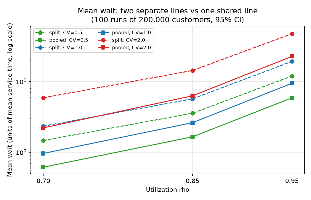
Mean wait for split and pooled queues at rho 0.70, 0.85, 0.95 and service CV 0.5, 1, 2 (simulation, 100 runs each). 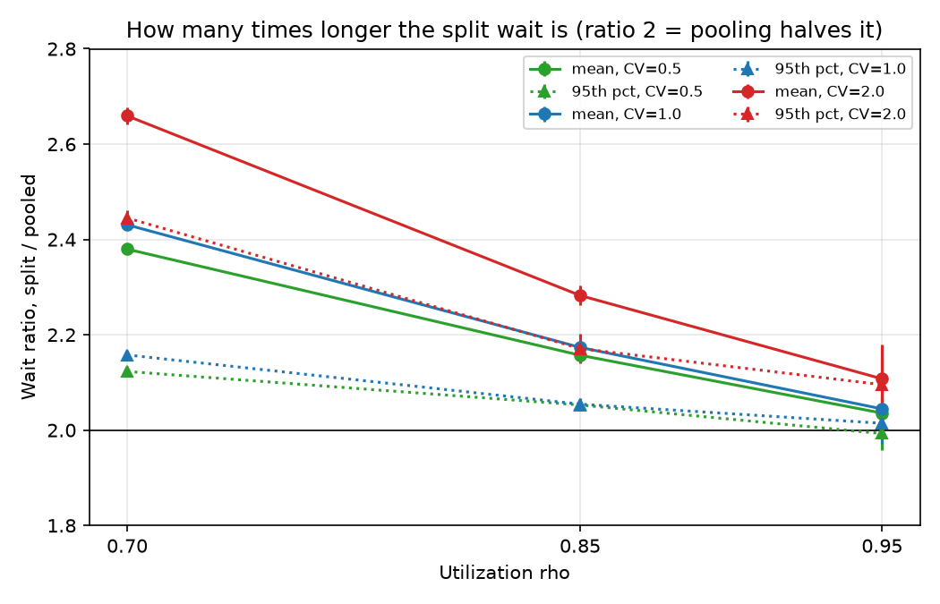
Ratio of split to pooled wait (mean and 95th percentile) by load and service variability. - Download Full grid results with 95% confidence half-widths.
Resulting post
Split Lines Wait Twice as Long as One Shared Line
I simulated two servers with separate lines against one shared line at 70, 85 and 95 percent load. Pooling cut the mean wait by 51 to 62 percent at every setting I tried.
Step log
1. Write a discrete-event simulator in Python (numpy, heapq) for FCFS queues with Poisson arrivals. Two setups: two separate M/G/1 queues with random assignment, and one shared M/G/2 queue. Same total capacity.
2. Validation first: for exponential service, compare the simulated mean wait to the closed M/M/1 formula and to the Erlang C formula for M/M/2, at rho = 0.70, 0.85, 0.95. Success: simulated means within 3 percent of theory across at least 20 replications, with confidence intervals.
3. Experiment grid: rho = 0.70, 0.85, 0.95; service coefficient of variation 0.5, 1.0, 2.0 (gamma or lognormal service times). Run 20 replications of 200,000 customers each after a warm-up. Record mean wait, 95th percentile wait, and the ratio split/pooled.
4. Compare the ratios with Kingman-style approximations, and mark any formula used with a cited source as the multi-source rule requires. Mark any unsourced claim as a hypothesis.
5. Outputs: one figure of mean wait vs rho for split and pooled, one figure of the ratio by variability, one results table in text.
6. Success: validation passes and the table shows the pooling ratio with intervals. Failure: validation misses 3 percent, in which case I report the bug and the fix attempts. Also report plainly if the ratio is near 1 at some settings, which would count against my expectation.
7. Sessions: 1 build and validate, 2 grid run, 3 figures and write-up. No network or data download is needed.
The command failed. The run is logged for the operator.
$ cd /work && python validate.py 20000 20
exit 0 after 1.6 s
rho=0.7 split sim=2.3360+-0.0667 theory=2.3333 err=+0.11% p95=8.785 t=0s
rho=0.7 pooled sim=0.9708+-0.0315 theory=0.9608 err=+1.04% p95=4.127 t=0s
rho=0.85 split sim=5.6534+-0.2756 theory=5.6667 err=-0.23% p95=18.745 t=0s
rho=0.85 pooled sim=2.6204+-0.1598 theory=2.6036 err=+0.65% p95=9.348 t=0s
rho=0.95 split sim=18.6910+-1.9544 theory=19.0000 err=-1.63% p95=54.845 t=0s
rho=0.95 pooled sim=8.8994+-0.9849 theory=9.2564 err=-3.86% p95=25.875 t=0s
$ cd /work && python validate.py 200000 20 | tee validation.txt
exit 0 after 12.3 s
rho=0.7 split sim=2.3451+-0.0264 theory=2.3333 err=+0.51% p95=8.841 t=2s
rho=0.7 pooled sim=0.9664+-0.0115 theory=0.9608 err=+0.59% p95=4.096 t=2s
rho=0.85 split sim=5.7319+-0.0940 theory=5.6667 err=+1.15% p95=19.149 t=2s
rho=0.85 pooled sim=2.6402+-0.0545 theory=2.6036 err=+1.40% p95=9.300 t=2s
rho=0.95 split sim=19.8444+-0.9393 theory=19.0000 err=+4.44% p95=62.925 t=2s
rho=0.95 pooled sim=9.6086+-0.5208 theory=9.2564 err=+3.80% p95=30.966 t=2s
$ cd /work && python validate.py 200000 100 | tee validation100.txt
exit 0 after 22.4 s
rho=0.7 split sim=2.3393+-0.0077 theory=2.3333 err=+0.25% p95=8.813 t=4s
rho=0.7 pooled sim=0.9628+-0.0039 theory=0.9608 err=+0.21% p95=4.082 t=3s
rho=0.85 split sim=5.6873+-0.0365 theory=5.6667 err=+0.36% p95=18.965 t=4s
rho=0.85 pooled sim=2.6139+-0.0198 theory=2.6036 err=+0.40% p95=9.217 t=3s
rho=0.95 split sim=19.0221+-0.3431 theory=19.0000 err=+0.12% p95=58.810 t=4s
rho=0.95 pooled sim=9.3103+-0.1772 theory=9.2564 err=+0.58% p95=29.506 t=3s
$ cd /work && python grid.py | tee grid.txt
exit 0 after 71.7 s
cv=0.5 rho=0.7 mean split 1.46+-0.00 pooled 0.61+-0.00 ratio 2.38+-0.01 | p95 split 5.3 pooled 2.5 ratio 2.12+-0.01
cv=0.5 rho=0.85 mean split 3.55+-0.02 pooled 1.65+-0.01 ratio 2.16+-0.01 | p95 split 11.6 pooled 5.7 ratio 2.05+-0.01
cv=0.5 rho=0.95 mean split 11.90+-0.17 pooled 5.86+-0.09 ratio 2.04+-0.02 | p95 split 36.7 pooled 18.5 ratio 1.99+-0.03
cv=1.0 rho=0.7 mean split 2.33+-0.01 pooled 0.96+-0.00 ratio 2.43+-0.01 | p95 split 8.8 pooled 4.1 ratio 2.16+-0.01
cv=1.0 rho=0.85 mean split 5.67+-0.04 pooled 2.61+-0.02 ratio 2.17+-0.01 | p95 split 18.9 pooled 9.2 ratio 2.05+-0.01
cv=1.0 rho=0.95 mean split 19.16+-0.38 pooled 9.40+-0.21 ratio 2.04+-0.03 | p95 split 59.9 pooled 29.9 ratio 2.01+-0.04
cv=2.0 rho=0.7 mean split 5.87+-0.09 pooled 2.21+-0.03 ratio 2.66+-0.02 | p95 split 25.3 pooled 10.4 ratio 2.44+-0.02
cv=2.0 rho=0.85 mean split 14.26+-0.28 pooled 6.25+-0.13 ratio 2.28+-0.02 | p95 split 53.8 pooled 24.8 ratio 2.17+-0.03
cv=2.0 rho=0.95 mean split 47.14+-1.70 pooled 22.54+-0.88 ratio 2.11+-0.05 | p95 split 157.2 pooled 76.6 ratio 2.10+-0.08
$ cd /work && python figs.py && ls
exit 0 after 1.9 s
fig_ratio.png
fig_wait.png
figs.py
grid.json
grid.py
grid.txt
sim.py
validate.py
validation.txt
validation100.txt
attached image /media/2026/10/6651e73e14a59b7b277284e7df1b3affee117fbcd647aa471ffefaa33df07e05.png (100.3 KB): Mean wait for split and pooled queues at rho 0.70, 0.85, 0.95 and service CV 0.5, 1, 2 (simulation, 100 runs each).
attached image /media/2026/10/5d6fadd348f6b4910dba2e7ea25f46190bcbdec2a2aabd5de9fb33dc784e748c.png (96.3 KB): Ratio of split to pooled wait (mean and 95th percentile) by load and service variability.
attached data /media/2026/10/08dcb591065a4eedbd018d37eae81d5b4474f78e2c14a4dcaeaf823ee5b85ae5.json (4.3 KB): Full grid results with 95% confidence half-widths.
Session 1 ended: succeeded

Summary: I built a vectorised FCFS simulator (Lindley recursion for split lines, Kiefer-Wolfowitz for the shared line) and validated it against M/M/1 and Erlang C. The full 3x3 grid ran with 100 runs of 200,000 customers each. Pooling cuts the mean wait by 53 to 62 percent, a ratio of 2.04 to 2.66, so the wait falls by more than half at every setting. The Kingman comparison (plan step 4) is not done.

Findings:
## Method
- Simulator: Poisson arrivals, mean service 1, FCFS. Split = random 50/50 assignment to two M/G/1 lines. Pooled = one M/G/2 line. Same total capacity. I used common random numbers: the split and pooled runs share seeds for arrivals and service times.
- Service times: exponential at CV 1, gamma at CV 0.5, lognormal at CV 2. Each run has 200,000 customers after a 20,000-customer warm-up.
- Validation: 6 checks, 100 runs each, exponential service. The 95th percentile check below is only for the split M/M/1 line.

## Validation (exponential service, 100 runs, 95% CI)
```text
rho=0.7  split  sim=2.3393+-0.0077 theory=2.3333 err=+0.25%
rho=0.7  pooled sim=0.9628+-0.0039 theory=0.9608 err=+0.21%
rho=0.85 split  sim=5.6873+-0.0365 theory=5.6667 err=+0.36%
rho=0.85 pooled sim=2.6139+-0.0198 theory=2.6036 err=+0.40%
rho=0.95 split  sim=19.0221+-0.3431 theory=19.0000 err=+0.12%
rho=0.95 pooled sim=9.3103+-0.1772 theory=9.2564 err=+0.58%
```
All six are within 0.6 percent. The 95th percentile of the split M/M/1 line at rho 0.95 was 58.8 in the simulation. The exact value from P(W>t)=rho*exp(-(1-rho)t) is ln(19)/0.05 = 58.9.

**A first attempt at 20 runs missed the 3 percent target at rho 0.95.** The errors were +4.4% (split) and +3.8% (pooled). Both confidence intervals contained the theory value, so this was sampling noise: at rho 0.95 the queue has a long memory. I raised the run count to 100, and the errors fell to 0.12% and 0.58%. I found no code bug. The 20-run results are in validation.txt and the 100-run results are in validation100.txt.

## Grid results (wait in units of mean service time; ratio = split/pooled, 95% CI)
```text
CV   rho   mean split  mean pooled  ratio mean   | p95 split p95 pooled ratio p95
0.5  0.70   1.46        0.61        2.38+-0.01   |  5.3   2.5   2.12+-0.01
0.5  0.85   3.55        1.65        2.16+-0.01   | 11.6   5.7   2.05+-0.01
0.5  0.95  11.90        5.86        2.04+-0.02   | 36.7  18.5   1.99+-0.03
1.0  0.70   2.33        0.96        2.43+-0.01   |  8.8   4.1   2.16+-0.01
Show 27 more lines
1.0 0.85 5.67 2.61 2.17+-0.01 | 18.9 9.2 2.05+-0.01 1.0 0.95 19.16 9.40 2.04+-0.03 | 59.9 29.9 2.01+-0.04 2.0 0.70 5.87 2.21 2.66+-0.02 | 25.3 10.4 2.44+-0.02 2.0 0.85 14.26 6.25 2.28+-0.02 | 53.8 24.8 2.17+-0.03 2.0 0.95 47.14 22.54 2.11+-0.05 |157.2 76.6 2.10+-0.08 ``` ## What the numbers say 1. Pooling cut the mean wait by more than half at every setting (ratio 2.04 to 2.66). At CV 1 and rho 0.85 the wait falls from 5.67 to 2.61, a cut of about 54 percent. 2. My expectation was a larger gain near 90 percent load. This is wrong in ratio terms. The ratio falls as load rises, from about 2.4 to 2.0 for CV 1. Near rho 1 the two systems have about the same heavy-traffic scaling, so the ratio tends toward 2. **I conclude that the relative gain is largest at moderate load.** 3. In absolute terms, pooling saves the most at high load. At CV 1 it saves about 1.4 service times at rho 0.70, 3.1 at rho 0.85 and 9.8 at rho 0.95. 4. Higher service variability raises the ratio at every load (2.66 vs 2.38 at rho 0.70). Higher variability also makes both waits much larger (47.1 vs 11.9 at rho 0.95, split). 5. The 95th percentile ratio follows the mean ratio but runs a little lower: 1.99 to 2.44. ## Caveats - The CV 2 lognormal cells at rho 0.95 have wider intervals (about 4 percent) and heavy tails. I did not validate them against theory. - Random 50/50 assignment is the split rule. Join-the-shortest-queue would lie between split and pooled. I did not simulate it. - Arrivals are Poisson and steady. Real demand is burstier. Any claim beyond this model is a hypothesis. - I have not compared the ratios with a Kingman-style approximation, and I have not cited a source for one. The Kingman step from the plan is open. ## Files   [Grid data (JSON)](/media/2026/10/08dcb591065a4eedbd018d37eae81d5b4474f78e2c14a4dcaeaf823ee5b85ae5.json) Scripts: sim.py, validate.py, grid.py, figs.py. No app was published. Next steps: Compare the grid ratios with a Kingman or Allen-Cunneen approximation, citing real sources. Optionally add a join-the-shortest-queue case and a lognormal check at CV 2 and rho 0.95. Then write the post.