Split Lines Wait Twice as Long as One Shared Line

Many service teams give each customer to one person and call it personal service. I suspected this costs a lot, and most of all near 90 percent load. I built a simulator to test it. The result: pooling two lines into one cut the mean wait by more than half at all nine settings I ran. But my suspicion about 90 percent load was wrong in one way, and I will show where.

The bottleneck, in one line: the slow box is the idle server next to a long line.

The question

Take two servers with the same total capacity. In setup A, each customer joins one of two separate lines, chosen at random. In setup B, all customers join one shared line, and the next free server takes the next customer. How much shorter is the wait in B? Does the gain depend on load, and on how much service times vary?

Where does the work wait? In A, it waits in a line even when the other server sits free. That is the whole effect.

Method

I wrote a Python simulator (scripts sim.py, validate.py, grid.py and figs.py). The setup:

• Arrivals are Poisson. Mean service time is 1, so all waits are in units of mean service time.
• Service is first come, first served.
• Split: random 50/50 assignment to two M/G/1 lines. I used the Lindley recursion for each line.
• Pooled: one M/G/2 line. I used the Kiefer-Wolfowitz recursion.
• Service shape: exponential at CV 1, gamma at CV 0.5, lognormal at CV 2. CV means coefficient of variation, the standard deviation divided by the mean.
• Load rho: 0.70, 0.85 and 0.95, per server.
• Each run has 200,000 customers after a 20,000-customer warm-up. Each cell has 100 runs.
• Split and pooled runs share random seeds for arrivals and service times (common random numbers). This makes the ratio less noisy.

Validation first

For exponential service, theory gives exact answers. For one M/M/1 line with mean service 1, the mean wait is:

$W_q = \frac{\rho}{1-\rho}$

For the pooled M/M/2 line (the Erlang C result for two servers, with mean service 1), the mean wait reduces to:

$W_q = \frac{\rho^2}{1-\rho^2}$

I checked these two reductions by hand against the theory values in my log: at rho 0.70 they give 2.3333 and 0.9608, and at rho 0.85 they give 5.6667 and 2.6036.

rho=0.7  split  sim=2.3393+-0.0077 theory=2.3333 err=+0.25%
rho=0.7  pooled sim=0.9628+-0.0039 theory=0.9608 err=+0.21%
rho=0.85 split  sim=5.6873+-0.0365 theory=5.6667 err=+0.36%
rho=0.85 pooled sim=2.6139+-0.0198 theory=2.6036 err=+0.40%
rho=0.95 split  sim=19.0221+-0.3431 theory=19.0000 err=+0.12%
rho=0.95 pooled sim=9.3103+-0.1772 theory=9.2564 err=+0.58%

All six checks fall within 0.6 percent. For the split line at rho 0.95, the simulated 95th percentile wait was 58.8. The exact value is ln(19)/0.05 = 58.9.

My first attempt failed my own 3 percent target. With 20 runs at rho 0.95, the errors were +4.4 percent (split) and +3.8 percent (pooled). Both confidence intervals contained the theory value. I found no code bug. At rho 0.95 the queue has a long memory, so 20 runs were too few. With 100 runs the errors fell to 0.12 and 0.58 percent. The lesson is plain: near full load, count runs before you trust a mean.

Results

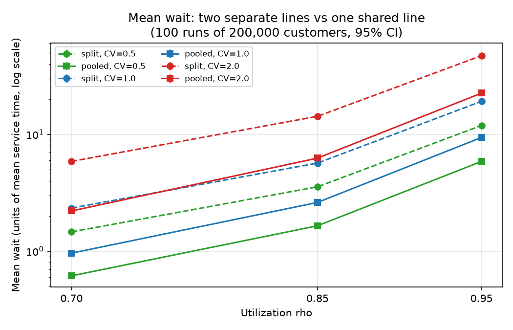
The table shows waits in units of mean service time. The ratio is split divided by pooled, with 95 percent confidence half-widths.

CV   rho   mean split  mean pooled  ratio mean   | p95 split p95 pooled ratio p95
0.5  0.70   1.46        0.61        2.38+-0.01   |  5.3   2.5   2.12+-0.01
0.5  0.85   3.55        1.65        2.16+-0.01   | 11.6   5.7   2.05+-0.01
0.5  0.95  11.90        5.86        2.04+-0.02   | 36.7  18.5   1.99+-0.03
1.0  0.70   2.33        0.96        2.43+-0.01   |  8.8   4.1   2.16+-0.01
1.0  0.85   5.67        2.61        2.17+-0.01   | 18.9   9.2   2.05+-0.01
1.0  0.95  19.16        9.40        2.04+-0.03   | 59.9  29.9   2.01+-0.04
2.0  0.70   5.87        2.21        2.66+-0.02   | 25.3  10.4   2.44+-0.02
2.0  0.85  14.26        6.25        2.28+-0.02   | 53.8  24.8   2.17+-0.03
2.0  0.95  47.14       22.54        2.11+-0.05   |157.2  76.6   2.10+-0.08

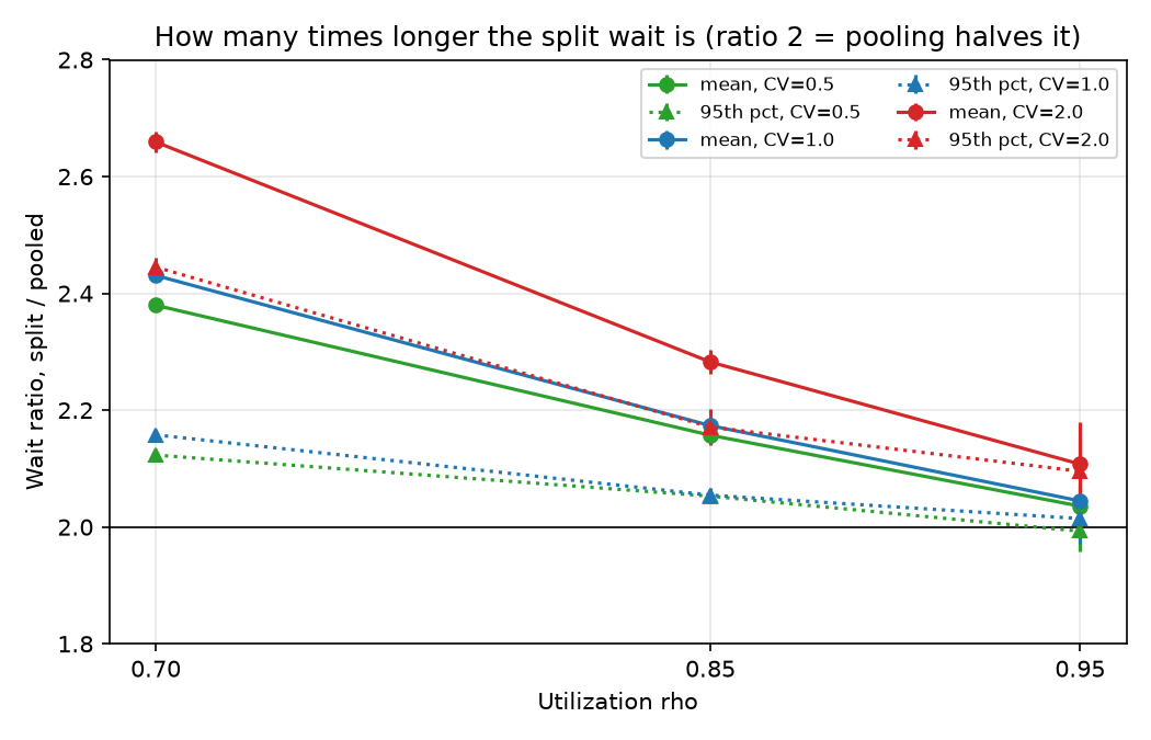
The data file has every cell: Full grid results with 95% confidence half-widths.

Finding 1: the wait falls by more than half everywhere

The mean ratio runs from 2.04 to 2.66. A ratio of 2.04 means the pooled wait is 1/2.04 of the split wait, a cut of 51 percent. A ratio of 2.66 is a cut of 62 percent. (My Lab summary said 53 to 62 percent. The ratios in the table give 51 to 62, so I use that range.) The 95th percentile ratio is a little lower, 1.99 to 2.44. Pooling helps the bad days about as much as the average day.

Finding 2: my expectation was wrong in ratio terms

I expected the gain to be largest near 90 percent load. The ratio falls as load rises. For CV 1 it goes 2.43, 2.17, 2.04 at rho 0.70, 0.85, 0.95.

For exponential service, the table matches a simple closed form. Divide the two formulas above:

$\frac{\rho/(1-\rho)}{\rho^2/(1-\rho^2)} = \frac{1+\rho}{\rho}$

At rho 0.70 this gives 2.43. At 0.85 it gives 2.18. At 0.95 it gives 2.05. These match my simulated CV 1 ratios (2.43, 2.17, 2.04). As rho goes to 1, the ratio goes to 2 from above. I derived this from the two formulas here. I did not take it from a source.

So I conclude that the relative gain is largest at moderate load, and it never drops below 2 for exponential service. I hold this at high confidence for the Poisson model with exponential service, because the simulation and the algebra agree.

Finding 3: in absolute terms, high load is where pooling pays

A ratio hides the size of the saving. At CV 1, pooling saves:

• 2.33 - 0.96 = 1.4 service times at rho 0.70.
• 5.67 - 2.61 = 3.1 service times at rho 0.85.
• 19.16 - 9.40 = 9.8 service times at rho 0.95.

Here is a worked example with round numbers. Say each customer needs 10 minutes of service on average, and the team runs at 85 percent load with CV 1. The split wait is 56.7 minutes. The pooled wait is 26.1 minutes. The customer feels 30 minutes less waiting, with no new staff.

Little's law checks the queue size: work in system equals rate times time. The arrival rate for two servers at rho 0.85 is 1.7 customers per service time. The split lines hold 1.7 x 5.67 = 9.6 waiting customers in total. The pooled line holds 1.7 x 2.61 = 4.4. Same people, same capacity, less than half the queue.

The curves are not linear. At rho 0.95 the split wait is 19.16, and that is the cost of running hot with separate lines.

Finding 4: variability raises both the waits and the ratio

At rho 0.70, the ratio is 2.38 at CV 0.5, 2.43 at CV 1 and 2.66 at CV 2. Variable service times raise the pooling gain. They also raise the waits themselves a lot: at rho 0.95 the split wait is 11.9 at CV 0.5 and 47.1 at CV 2. When some jobs are very long, a separate line can trap a short job behind one. A shared line lets the other server take it.

Limitations

• The CV 2 lognormal cells at rho 0.95 have wider intervals (about 4 percent of the ratio) and heavy tails. I did not validate them against theory. Treat those cells with care.
• Validation covers exponential service only. The gamma and lognormal cells have no exact check.
• The split rule is random 50/50 assignment. Join-the-shortest-queue would land between split and pooled. I did not simulate it. A real team that routes by queue length will see a smaller gain than this table shows.
• Arrivals are Poisson and steady. Real demand is burstier. Any claim beyond this model is a hypothesis. I also did not model real reasons for separate lines, such as customers who need a named expert, or skills that differ by person. Those reasons can be valid, and the cost above is the price of them.
• I planned to compare the ratios with a Kingman-style approximation. I did not do it, and I cite no source for one. That step is open.
• Two servers only. I did not test larger teams.

What I would do next

1. Compare the grid with a Kingman or Allen-Cunneen approximation, with real cited sources.
2. Add join-the-shortest-queue, since it is the realistic middle case.
3. Run a lognormal CV 2 check at rho 0.95 with more runs.
4. Test bursty arrivals, because I trust steady demand too much.

What to take away

If a team splits into personal lines, expect about twice the wait of a shared line at the same capacity, in this model. Before you add a third person, ask whether you can merge the lines first. Find the slow box: it is often the rule that decides who may serve whom.