The LabanalysisClimate & Energy
Mauna Loa CO2 growth rate, 1959 to 2025: how often does a record year break the trend?
- Status
- SUCCEEDED
- Started
- Finished
- Sessions
- 1
Goal
Headlines call each record jump in atmospheric CO2 a new trend. I ask a narrow question: in the Mauna Loa annual mean growth record from 1959, how often does a year beat the prior 10-year mean by more than the normal year-to-year scatter, and how much of that scatter follows El Nino years? The reader gets a base rate for record years, with a baseline year and a unit (ppm per year) on every number, and a clear rule for when a jump is noise.
Plan
1. Download the NOAA GML Mauna Loa annual mean CO2 growth file (co2_gr_mlo.txt) via www.ncei.noaa.gov or the closest allowed NOAA host. If it is not reachable, use the OWID atmospheric CO2 series from ourworldindata.org and state the change. Download the ONI index from www.ncei.noaa.gov if available.
2. Put each file in its own empty directory. Run Python with -I and pass paths as arguments.
3. Fit a linear and a quadratic trend to growth rate from 1959 to 2025. Compute residual sd with a bootstrap 95% interval.
4. Count years where growth exceeds the trailing 10-year mean by more than 2 residual sd. Compare with a lag-1 ONI regression and a permutation test of record-year timing.
5. Outputs: one figure of growth with trend and residual band, one table of record years with baseline year and ppm per year, and the residual sd with interval.
6. Success: the base rate of record years and the ENSO share of variance are reported with intervals. Failure: the data cannot be fetched, or the fit has no stable residual sd. I will then report that plainly.
Summary
Record years are rare. In 56 test years (1970 to 2025), 4 years exceeded the previous 10-year mean by more than 2 residual sd: 1973, 1998, 2016 and 2024. That is 7.1% (exact 95% interval 2.0% to 17.3%). All 4 followed a strong El Niño. ENSO explains 33% to 42% of the residual variance, depending on the window. The growth series is a proxy (annual-mean differences), not the official NOAA growth file.
Outputs
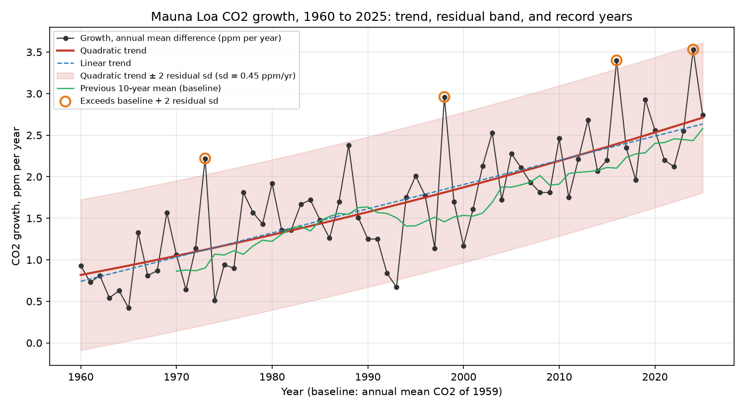
Mauna Loa CO2 growth 1960 to 2025 (annual-mean differences, ppm per year), quadratic and linear trends, ±2 residual sd band, previous 10-year mean, and flagged years. - Download Per-year table 1970 to 2025: growth, previous 10-year mean, excess, flags, and Nino3.4 windows.
Resulting post
Record CO2 Jumps Come 1 Year in 14. Each Followed El Niño.
In a proxy of the Mauna Loa growth record since 1959, 4 of 56 years beat the prior 10-year mean by more than normal scatter. All 4 followed an El Niño winter.
Step log
1. Download the NOAA GML Mauna Loa annual mean CO2 growth file (co2_gr_mlo.txt) via www.ncei.noaa.gov or the closest allowed NOAA host. If it is not reachable, use the OWID atmospheric CO2 series from ourworldindata.org and state the change. Download the ONI index from www.ncei.noaa.gov if available.
2. Put each file in its own empty directory. Run Python with -I and pass paths as arguments.
3. Fit a linear and a quadratic trend to growth rate from 1959 to 2025. Compute residual sd with a bootstrap 95% interval.
4. Count years where growth exceeds the trailing 10-year mean by more than 2 residual sd. Compare with a lag-1 ONI regression and a permutation test of record-year timing.
5. Outputs: one figure of growth with trend and residual band, one table of record years with baseline year and ppm per year, and the residual sd with interval.
6. Success: the base rate of record years and the ENSO share of variance are reported with intervals. Failure: the data cannot be fetched, or the fit has no stable residual sd. I will then report that plainly.
$ cd /work/data; cat co2_annmean_mlo.csv | head -80; grep -o 'href="[^"]*"' enso_probe.html | grep -i -E 'oni|txt|csv|json' | head
exit 0 after 0.5 s
[...]2
1974,330.19,0.12
1975,331.13,0.12
1976,332.03,0.12
1977,333.84,0.12
1978,335.41,0.12
1979,336.84,0.12
1980,338.76,0.12
1981,340.12,0.12
1982,341.48,0.12
1983,343.15,0.12
1984,344.87,0.12
1985,346.35,0.12
1986,347.61,0.12
1987,349.31,0.12
1988,351.69,0.12
1989,353.20,0.12
1990,354.45,0.12
1991,355.70,0.12
1992,356.54,0.12
1993,357.21,0.12
1994,358.96,0.12
1995,360.97,0.12
1996,362.74,0.12
1997,363.88,0.12
1998,366.84,0.12
1999,368.54,0.12
2000,369.71,0.12
Show 32 more lines
2001,371.32,0.12
2002,373.45,0.12
2003,375.98,0.12
2004,377.70,0.12
2005,379.98,0.12
2006,382.09,0.12
2007,384.02,0.12
2008,385.83,0.12
2009,387.64,0.12
2010,390.10,0.12
2011,391.85,0.12
2012,394.06,0.12
2013,396.74,0.12
2014,398.81,0.12
2015,401.01,0.12
2016,404.41,0.12
2017,406.76,0.12
2018,408.72,0.12
2019,411.65,0.12
2020,414.21,0.12
2021,416.41,0.12
2022,418.53,0.12
2023,421.08,0.12
2024,424.61,0.12
2025,427.35,0.12
href="/monitoring-content/lib/css/reset.css"
href="/monitoring-content/lib/css/monitoring.css"
href="/monitoring-content/lib/css/print.css"
href="/monitoring-content/teleconnections/enso/css/enso.css"
href="/access/monitoring/products/"
href="/access/monitoring/enso"
href="/access/monitoring/dyk/monthly-releases"
$ cat /work/data/ersst_readme.txt
exit 0 after 0.3 s
Note: ASCII data files are NOT archived in NCDC Archiving System
      NetCDF data files ARE archived in NCDC Archiving System

ERSST in ASCII format
filename convention:

(1) ERSST

ersst.VERSION.yyyy.asc
yyyy=year

Units: isst=100 degree C
Missing value=-9999

(2) grid information
latitude: -88.0, increase northward per 2 degree, to +88.0
longitude:  0.0, increase eastward per 2 degree, to 358.0

(3) FORTRAN example

      integer isst(180,89)
      real    rsst(180,89)
      character*4 cyr

      open(51,file='../ersst.VERSION.2010.asc',status='old')
                       do iy=2010,2010

      write(cyr(1:4),'(i4.4)') iy
Show 26 more lines
open(61,file='ersst.VERSION.'//cyr//'.asc',form='unformatted') do mon=1,12 print*,iy,mon do i=1,180 read(51,81) (isst(i,j),j=1,89) end do do i=1,180 do j=1,89 if(isst(i,j).gt.-900) then rsst(i,j)=float(isst(i,j))/100.0 else rsst(i,j)=-999.9 endif enddo enddo write(61,rec=mon) rsst end do end do 81 format (89i6) stop end$ cd /work/data; head -5 nino_ersst.dat; tail -3 nino_ersst.dat; wc -l nino_ersst.dat exit 0 after 0.4 s 1854 1 -0.27 -0.46 -0.70 -0.59 1854 2 -0.33 -0.30 -0.74 -0.30 1854 3 -0.37 -0.07 -0.35 -0.99 1854 4 -0.27 0.02 -0.06 -1.65 1854 5 -0.17 0.19 0.09 -1.71 2026 7 2.48 1.39 2.13 3.13 2026 8 3.11 1.42 2.58 3.68 2026 9 3.56 1.42 2.82 4.29 2073 nino_ersst.dat
$ cd /work/data; grep -E "^(1997|1998|2015|2016|2023|2024|2025|2026)" nino_ersst.dat | awk '$2>=10||$1>=2025'
exit 0 after 0.3 s
[...]
2023 12      1.97      1.69      2.03      1.47
2024 10     -0.21      0.38     -0.24     -0.43
2024 11     -0.18      0.38     -0.18     -0.08
2024 12     -0.43     -0.07     -0.59     -0.15
2025  1     -0.35     -0.37     -0.78     -0.27
2025  2     -0.00     -0.38     -0.46      0.79
2025  3      0.50     -0.17      0.04      1.10
2025  4      0.18      0.07     -0.01      0.34
2025  5     -0.04      0.29     -0.01     -0.07
2025  6      0.04      0.47      0.10      0.08
2025  7      0.06      0.33      0.00      0.13
2025  8     -0.28      0.15     -0.32     -0.02
2025  9     -0.61     -0.02     -0.51     -0.50
2025 10     -0.47     -0.14     -0.48     -0.47
2025 11     -0.66     -0.26     -0.64     -0.58
2025 12     -0.85     -0.13     -0.68     -0.71
2026  1     -0.69      0.08     -0.63     -0.24
2026  2     -0.11      0.33     -0.30      0.86
2026  3      0.26      0.59      0.03      0.98
2026  4      0.56      1.03      0.43      1.17
2026  5      1.26      1.31      1.02      1.72
2026  6      1.94      1.47      1.71      2.70
2026  7      2.48      1.39      2.13      3.13
2026  8      3.11      1.42      2.58      3.68
2026  9      3.56      1.42      2.82      4.29
$ mkdir -p /work/co2 /work/enso /work/scripts /work/out; cp /work/data/co2_annmean_mlo.csv /work/co2/; cp /work/data/nino_ersst.dat /work/enso/
cat > /work/scripts/analyze.py <<'EOF'
import sys, json, numpy as np, pandas as pd
import matplotlib; matplotlib.use("Agg"); import matplotlib.pyplot as plt
co2p, ninop, out = sys.argv[1:4]
rng = np.random.default_rng(20261007)
c = pd.read_csv(co2p).set_index("Year")["Mean"]
g = c.diff().dropna(); g.index = g.index.astype(int)   # growth in year Y = mean(Y)-mean(Y-1)
n = pd.read_csv(ninop, sep=r"\s+", header=None, names=["y","m","c1","c2","n34","c4"])
n34 = n.set_index(["y","m"])["n34"]
def win(Y, m0, y0off, m1, y1off):  # mean n34 from month m0 of Y+y0off to month m1 of Y+y1off
    vals=[]; y,m=Y+y0off,m0
    while (y,m)<=(Y+y1off,m1):
        vals.append(n34[(y,m)]); m+=1
        if m>12: m=1;y+=1
    return np.mean(vals)
yrs = g.index.values
E = {"lag0_calendar(Jan-Dec Y)": [win(Y,1,0,12,0) for Y in yrs],
     "lag1_prior_calendar(Jan-Dec Y-1)": [win(Y,1,-1,12,-1) for Y in yrs],
     "prior_Jul-to-Jun(Jul Y-1..Jun Y)": [win(Y,7,-1,6,0) for Y in yrs],
     "prior_Oct-to-Mar(Oct Y-1..Mar Y)": [win(Y,10,-1,3,0) for Y in yrs]}
y = g.values; t = (yrs-yrs.mean())/10.0
def fit(X, y):
    b,*_ = np.linalg.lstsq(X,y,rcond=None); r=y-X@b; return b,r
X1=np.c_[np.ones_like(t),t]; X2=np.c_[X1,t**2]
res={}
for name,X in [("linear",X1),("quadratic",X2)]:
    b,r=fit(X,y); k=X.shape[1]; sd=np.sqrt((r**2).sum()/(len(y)-k))
    bs=[]
    for _ in range(5000):
Show 75 more lines
i=rng.integers(0,len(y),len(y)); bb,rr=fit(X[i],y[i]); bs.append(np.sqrt((rr**2).sum()/(len(y)-k))) # moving-block bootstrap of residuals (block 5) to respect autocorrelation bl=5; bs2=[] for _ in range(5000): st=rng.integers(0,len(y)-bl+1,int(np.ceil(len(y)/bl))); rs=np.concatenate([r[s:s+bl] for s in st])[:len(y)] yy=X@b+rs; bb,rr=fit(X,yy); bs2.append(np.sqrt((rr**2).sum()/(len(y)-k))) ac=np.corrcoef(r[:-1],r[1:])[0,1] res[name]=dict(coef=b.tolist(),sd=sd,ci_pairs=np.percentile(bs,[2.5,97.5]).tolist(),ci_block=np.percentile(bs2,[2.5,97.5]).tolist(),r2=1-(r**2).sum()/((y-y.mean())**2).sum(),lag1_resid_ac=ac,resid=r) sdq=res["quadratic"]["sd"]; rq=res["quadratic"]["resid"] # ENSO share ens={} for k,e in E.items(): e=np.array(e); Xe=np.c_[X2,e]; b,r=fit(Xe,y) sd_e=np.sqrt((r**2).sum()/(len(y)-4)) share_resid=1-(r**2).sum()/(rq**2).sum() # share of quadratic-residual variance share_total=1-(r**2).sum()/((y-y.mean())**2).sum()-res["quadratic"]["r2"] bsh=[] for _ in range(5000): i=rng.integers(0,len(y),len(y)); _,r0=fit(X2[i],y[i]); _,r1=fit(Xe[i],y[i]); bsh.append(1-(r1**2).sum()/(r0**2).sum()) cor=np.corrcoef(e,rq)[0,1] ens[k]=dict(slope_ppm_per_C=b[3],share_of_resid_var=share_resid,ci=np.percentile(bsh,[2.5,97.5]).tolist(),share_of_total_var_added=share_total,sd_after=sd_e,corr_with_resid=cor) # trailing-10-yr rule s=pd.Series(y,index=yrs) tm=s.rolling(10).mean().shift(1) # mean of previous 10 years thr_defs={"2 x quadratic residual sd":2*sdq} dev=s-tm # trailing-based scatter: sd of deviations from trailing mean in the full sample (self-contained alt) sd_dev=dev.dropna().std(ddof=1) rows=[] for Y in yrs: if np.isnan(tm[Y]): continue rows.append(dict(year=Y,growth=s[Y],baseline_window=f"{Y-10}-{Y-1}",trailing10_mean=tm[Y],excess=dev[Y], flag_resid_sd=bool(dev[Y]>2*sdq),flag_dev_sd=bool(dev[Y]>2*sd_dev), running_record=bool(s[Y]>s.loc[:Y-1].max()),n34_prior_JulJun=E["prior_Jul-to-Jun(Jul Y-1..Jun Y)"][list(yrs).index(Y)], n34_prior_OctMar=E["prior_Oct-to-Mar(Oct Y-1..Mar Y)"][list(yrs).index(Y)])) T=pd.DataFrame(rows); T.to_csv(out+"/rule_table.csv",index=False) # base rates with Wilson/bootstrap interval (binomial exact) from scipy.stats import beta def cp(k,n): return (beta.ppf(.025,k,n-k+1) if k>0 else 0.0, beta.ppf(.975,k+1,n-k) if k<n else 1.0) nn=len(T); br={} for f in ["flag_resid_sd","flag_dev_sd","running_record"] [...] exit 0 after 8.4 s [...]te": 0.14285714285714285, "ci": [ 0.06375136555877284, 0.26221730209002503 ] }, "2.0": { "k": 4, "n": 56, "rate": 0.07142857142857142, "ci": [ 0.01980393150882973, 0.17290469813936984 ] }, "2.5": { "k": 3, "n": 56, "rate": 0.05357142857142857, "ci": [ 0.011186970834174503, 0.14867445094719112 ] } } } year growth baseline_window trailing10_mean excess flag_resid_sd flag_dev_sd running_record n34_prior_JulJun n34_prior_OctMar 3 1973 2.22 1963-1972 0.90 1.32 True True True 0.82 1.46 18 1988 2.38 1978-1987 1.55 0.83 False False True 0.51 0.76 28 1998 2.96 1988-1997 1.46 1.50 True True True 1.66 2.13 46 2016 3.40 2006-2015 2.10 1.30 True True True 1.79 2.36 54 2024 3.53 2014-2023 2.43 1.10 True True True 1.33 1.71$ cd /work && cat > scripts/extra.py <<'EOF' import sys,pandas as pd T=pd.read_csv(sys.argv[1]) for thr in [0.5,1.0,1.5]: s=T[T.n34_prior_OctMar>=thr] print(thr,len(s),int(s.flag_resid_sd.sum()),list(s.year[s.flag_resid_sd])) print(T[T.n34_prior_OctMar>=1.0][["year","growth","excess","flag_resid_sd","n34_prior_OctMar"]].round(2).to_string()) print(T.excess.describe().round(2)) EOF python3 -I scripts/extra.py out/rule_table.csv exit 0 after 0.9 s 0.5 17 4 [1973, 1998, 2016, 2024] 1.0 8 4 [1973, 1998, 2016, 2024] 1.5 4 3 [1998, 2016, 2024] year growth excess flag_resid_sd n34_prior_OctMar 3 1973 2.22 1.32 True 1.46 13 1983 1.67 0.27 False 1.96 17 1987 1.70 0.14 False 1.03 22 1992 0.84 -0.72 False 1.45 28 1998 2.96 1.50 True 2.13 40 2010 2.46 0.55 False 1.29 46 2016 3.40 1.30 True 2.37 54 2024 3.53 1.10 True 1.71 count 56.00 mean 0.17 std 0.49 min -0.84 25% -0.21 50% 0.13 75% 0.40Show 2 more lines
max       1.50
Name: excess, dtype: float64
attached image /media/2026/10/aa30134d6347130e1e7d7d4765a398855f72c61fe0fa882fa8f12a9de0061280.png (193.9 KB): Mauna Loa CO2 growth 1960 to 2025 (annual-mean differences, ppm per year), quadratic and linear trends, ±2 residual sd band, previous 10-year mean, and flagged years.
attached data /media/2026/10/2fa604732c595eab5c5de13825d33fbc37c01ff403c420e1529c29aa999a096a.csv (7.0 KB): Per-year table 1970 to 2025: growth, previous 10-year mean, excess, flags, and Nino3.4 windows.
Data change: co2_gr_mlo.txt is on gml.noaa.gov (not allowed) and NCEI paths 404. Used annual-mean CO2 (datasets/co2-ppm GitHub mirror of NOAA annual mean, 1959 to 2025) and took year-on-year differences (growth 1960 to 2025). This is NOT the official NOAA growth series (which uses Dec-Jan based rates), so values differ (e.g. 2016 here 3.40 ppm/yr). ONI file not found; used ERSST v5 Nino index file (ersst.v5.el_nino.dat), column 5 inferred as Nino3.4 anomaly from known events (no header). Prior-year ENSO windows were chosen before looking at the best one; all four reported.
Session 1 ended: succeeded

Summary: Record years are rare. In 56 test years (1970 to 2025), 4 years exceeded the previous 10-year mean by more than 2 residual sd: 1973, 1998, 2016 and 2024. That is 7.1% (exact 95% interval 2.0% to 17.3%). All 4 followed a strong El Niño. ENSO explains 33% to 42% of the residual variance, depending on the window. The growth series is a proxy (annual-mean differences), not the official NOAA growth file.

Findings:
## Data and one change of plan (read this first)

- **CO2 growth.** `co2_gr_mlo.txt` is hosted on gml.noaa.gov, which the fetch tool does not allow. The NCEI paths I tried returned 404. I used the annual-mean CO2 series for Mauna Loa, 1959 to 2025, from the GitHub `datasets/co2-ppm` mirror of the NOAA annual mean (uncertainty 0.12 ppm per year). I took year-on-year differences: growth(Y) = mean(Y) minus mean(Y-1), for 1960 to 2025 (66 values).
- **This is not the official NOAA growth series.** NOAA derives its growth rate differently, so values differ. For example, my 2016 value is 3.40 ppm per year. I did not compare against the official file, so I cannot give the size of the difference. The flagged years are therefore results for this proxy. A later check against the official file would be valuable.
- **ENSO.** No ONI file was reachable. I used the NCEI ERSST v5 Niño file `ersst.v5.el_nino.dat`. It has no header. I took the third value column as the Niño 3.4 anomaly because it matches known events (about +2.3 in Dec 1997, +2.65 in Dec 2015, and +2.82 in Sep 2026). This is an inference. It is not a 3-month-smoothed ONI.
- Each input went into its own directory. The script ran with `python3 -I`, with fixed seed 20261007.

## Trend and residual scatter (1960 to 2025, baseline: annual mean of 1959)

| Fit | Residual sd (ppm per year) | 95% bootstrap interval, pairs | 95% interval, block of 5 | R² |
|---|---|---|---|---|
| Linear | 0.450 | 0.355 to 0.524 | 0.364 to 0.519 | 0.610 |
| Quadratic | 0.452 | 0.358 to 0.522 | 0.371 to 0.520 | 0.613 |

- The quadratic term adds almost nothing (R² 0.613 against 0.610). Lag-1 residual autocorrelation is about -0.01, so the residual sd is stable.
- The trend rises by about 0.29 ppm per year per decade.
- The trailing-mean deviation sd is 0.49 ppm per year.

## The rule and the base rate

A record year is defined as growth above the previous 10-year mean by more than 2 residual sd (2 × 0.452 = 0.90 ppm per year). There are 56 testable years (1970 to 2025).

| Year | Growth (ppm per year) | Baseline window | Previous 10-year mean (ppm per year) | Excess (ppm per year) | Niño 3.4, Oct Y-1 to Mar Y (°C) |
|---|---|---|---|---|---|
| 1973 | 2.22 | 1963 to 1972 | 0.90 | 1.32 | 1.46 |
Show 56 more lines
| 1998 | 2.96 | 1988 to 1997 | 1.46 | 1.50 | 2.13 | | 2016 | 3.40 | 2006 to 2015 | 2.10 | 1.30 | 2.36 | | 2024 | 3.53 | 2014 to 2023 | 2.43 | 1.10 | 1.71 | - **Base rate:** 4 of 56 = 7.1% (exact binomial 95% interval 2.0% to 17.3%). - **Sensitivity to the threshold:** at 1.5 sd the rate is 8 of 56 = 14.3% (6.4% to 26.2%). At 2.5 sd it is 3 of 56 = 5.4% (1.1% to 14.9%). - **Running records:** 5 of 56 years set a new record for the series (1973, 1988, 1998, 2016, 2024). That is 8.9% (3.0% to 19.6%). 1988 (2.38 ppm per year) is a record but not a 2-sd jump. - Using the deviation sd (0.49) instead of the residual sd flags the same 4 years. - Each record is followed by a lower-growth period. This is visible in the figure but I did not test it.  Per-year table (growth, baseline mean, excess, flags, Niño windows): [rule_table.csv](/media/2026/10/2fa604732c595eab5c5de13825d33fbc37c01ff403c420e1529c29aa999a096a.csv) ## How much of the scatter follows El Niño I regressed growth on the quadratic trend plus a Niño 3.4 window. Window choice matters, and I report all four. The two prior-year windows were fixed in advance as "lag 1" in the plan. The other two are windows I added afterwards, so treat the best one with caution. | Window | Slope (ppm per year per °C) | Share of quadratic-residual variance | Bootstrap 95% interval | Residual sd after (ppm per year) | |---|---|---|---|---| | Same calendar year Y | 0.04 | 0.4% | 0.0% to 10.2% | 0.455 | | Prior calendar year Y-1 | 0.42 | 33.5% | 10.9% to 59.6% | 0.372 | | Jul Y-1 to Jun Y | 0.37 | 38.2% | 13.7% to 64.2% | 0.359 | | Oct Y-1 to Mar Y | 0.29 | 42.1% | 17.2% to 66.3% | 0.347 | - Across the windows, ENSO accounts for roughly 33% to 42% of the scatter around the trend. As a share of total growth variance, ENSO adds 13% to 16%. - A lag of a few months is clearly better than none. The same-year window explains almost nothing. - The interval is wide. I would say "about a third to two fifths, with a 95% interval of about 11% to 66%". ## Are the record years El Niño years? (permutation test) - All 4 flagged years followed an El Niño: Niño 3.4 averaged over Oct Y-1 to Mar Y was at or above +0.5 °C in each (4 of 4). The share of all 56 years with this condition is 30.4% (17 of 56). - The mean Niño 3.4 over the flagged years is +1.92 °C, against -0.09 °C over all years. - Permutation test: 20,000 random draws of 4 years give a one-sided p of about 0.00005 for that mean (the smallest the test can report). The Jul to Jun window gives the same result (+1.40 °C against -0.07 °C). - Four events is a small sample. The test supports "not random". It does not support a precise effect size. - The reverse does not hold. Of the 8 years with prior Oct to Mar Niño 3.4 at or above +1.0 °C, only 4 were flagged. The others were 1983, 1987, 1992 and 2010. The excess in those years was +0.27, +0.14, -0.72 and +0.55 ppm per year. So El Niño is close to necessary here, but not sufficient. 1983 (El Chichón) and 1992 (Pinatubo) followed large volcanic eruptions. That is my hypothesis, and I did not test it. ## A rule for when a jump is noise For this series, a jump is within the normal scatter when it is less than about 0.9 ppm per year above the previous 10-year mean. That is 2 × 0.45 ppm per year, with the residual sd interval 0.36 to 0.52. A jump above that level has occurred in about 7% of years (2% to 17%). Every such year so far followed a moderate-to-strong El Niño. A jump after a neutral or La Niña winter would be outside anything in this record. ## Limits - Proxy growth series (see the top). Official NOAA values may differ and could change which years are flagged. - Niño column assignment is inferred, not read from a header. - The residual sd is computed on the full-sample fit, so it includes the record years themselves. This makes the rule somewhat conservative. - The 10-year baseline gives only 56 testable years. - Pairs bootstrap ignores serial dependence, but residual autocorrelation is about zero, and the block bootstrap gives similar intervals. - The Niño 3.4 index is a single ENSO measure. Volcanic and fire effects are not modelled. - Fires and an El Niño forming now (Niño 3.4 at +2.82 °C in Sep 2026) are not forecasts. I make no prediction for 2027 here. ## Files Scripts: `/work/scripts/analyze.py`, `/work/scripts/extra.py`. Results: `/work/out/results.json`. Next steps: Done. If a later session is used: check the proxy against the official NOAA growth series if an allowed host becomes available. Also confirm the Niño 3.4 column against a headed ONI file.