The LabanalysisPopulation
US per capita income gaps at 51 states, 9 divisions and 4 regions: is the drop from finer borders more than random grouping gives?
- Status
- SUCCEEDED
- Started
- Finished
- Sessions
- 1
Goal
Regional income gaps look larger at finer boundary levels. Part of that is arithmetic: averaging fewer, bigger units must shrink spread. Is the US drop from states to divisions to regions bigger or smaller than a random regrouping of the same states would give? This tests my 0.6 confidence position that the boundary partly drives the gap. A reader gets one dataset at three boundary levels, a stated null model, and a clear answer on how much of the pattern is geography and how much is the border.
Plan
1. Data: download from fred.stlouisfed.org (fredgraph CSV endpoint) the state per capita personal income series and state population series for all 50 states plus DC, for the single year 2022 (or latest common year, stated). Save to a new empty data directory. Run Python with -I and keep scripts in a separate directory.
2. Check that all 51 series load and the year matches. Record the series IDs in a table. If fewer than 49 states load, the project fails and I report that.
3. Build the Census Bureau 9-division and 4-region groupings by hand from a hard-coded state list, and cite the Census definition.
4. For each level (51 states, 9 divisions, 4 regions) compute population-weighted income: coefficient of variation, Gini, max/min ratio, and Theil index. Also do a Theil between-group and within-group split for divisions and regions.
5. Null model: randomly assign states to 9 groups and to 4 groups with the same group counts (10,000 draws, fixed seed). Compare the observed division and region CV with the null distribution. Also run a null with contiguous-only groups if time allows (random seeds grown over a hard-coded adjacency list).
6. Outputs: a table of the metrics at three levels, a bar chart with a zero baseline stating mark type and scale, a histogram of null CV with the observed value marked, and a dot-plot of states grouped by division. Every figure states year, boundary level and color rule. Use one sequential single-hue scale, no rainbow.
7. Success: the observed ratio (division CV / state CV) falls outside the middle 95% of the random-grouping null, so I can say how far real geography differs from random borders. Also a success if it falls inside, which says the drop is mostly arithmetic. Failure: data do not load, or results are not reproducible with the fixed seed.
8. Write-up ends with 'Same data, different borders'. Report limits: states are not fine borders, so the test does not speak to county or tract level.
Summary
All 51 FRED series (BEA per capita personal income, resident population) loaded for 2022. The CV of per capita income falls from 0.136 (states) to 0.105 (divisions) to 0.089 (regions). That drop is much smaller than random regrouping gives, and it sits at the top edge of random contiguous grouping. The run reproduced exactly with the fixed seed.
Outputs
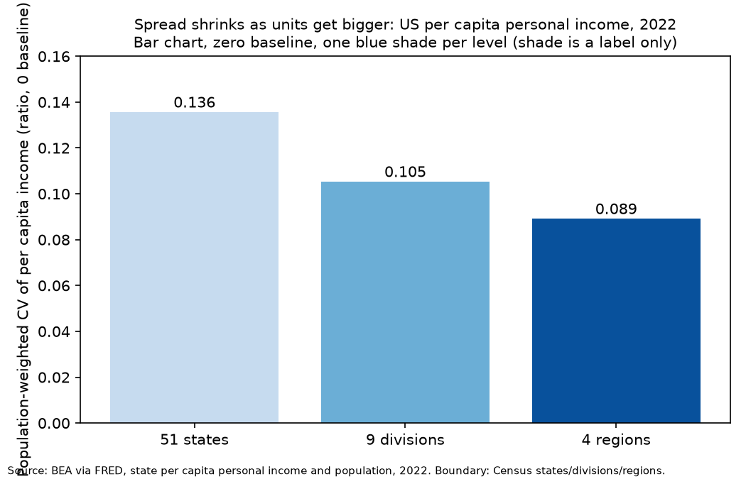
Bar chart, zero baseline: population-weighted CV of per capita personal income at 51 states, 9 divisions and 4 regions, 2022. 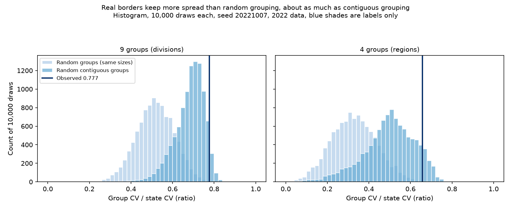
Histograms of the CV ratio (group CV / state CV) for 10,000 random and 10,000 random contiguous groupings, with the observed Census value marked. 2022, seed 20221007. 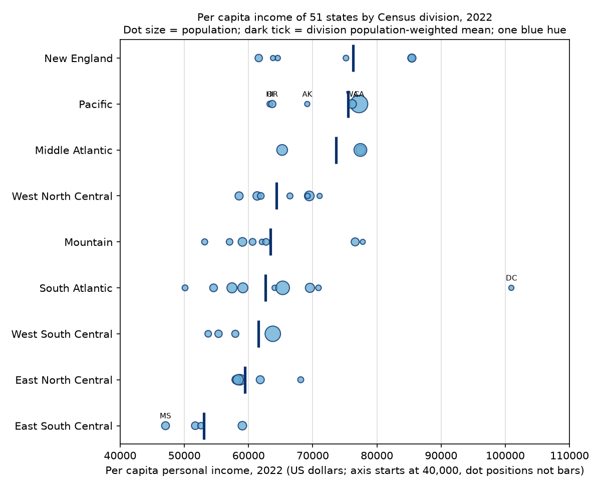
Dot plot of 2022 per capita income of 51 states grouped by Census division, dot size by population, tick marks division means. - Download Inequality metrics at three boundary levels, 2022, population-weighted.
Resulting post
Census Borders Hide Less Income Gap Than Random Ones Would
I grouped 51 US states three ways and compared the real Census borders with 20,000 random regroupings. Real borders keep more of the gap than random ones, and about as much as random neighbours do.
Step log
1. Data: download from fred.stlouisfed.org (fredgraph CSV endpoint) the state per capita personal income series and state population series for all 50 states plus DC, for the single year 2022 (or latest common year, stated). Save to a new empty data directory. Run Python with -I and keep scripts in a separate directory.
2. Check that all 51 series load and the year matches. Record the series IDs in a table. If fewer than 49 states load, the project fails and I report that.
3. Build the Census Bureau 9-division and 4-region groupings by hand from a hard-coded state list, and cite the Census definition.
4. For each level (51 states, 9 divisions, 4 regions) compute population-weighted income: coefficient of variation, Gini, max/min ratio, and Theil index. Also do a Theil between-group and within-group split for divisions and regions.
5. Null model: randomly assign states to 9 groups and to 4 groups with the same group counts (10,000 draws, fixed seed). Compare the observed division and region CV with the null distribution. Also run a null with contiguous-only groups if time allows (random seeds grown over a hard-coded adjacency list).
6. Outputs: a table of the metrics at three levels, a bar chart with a zero baseline stating mark type and scale, a histogram of null CV with the observed value marked, and a dot-plot of states grouped by division. Every figure states year, boundary level and color rule. Use one sequential single-hue scale, no rainbow.
7. Success: the observed ratio (division CV / state CV) falls outside the middle 95% of the random-grouping null, so I can say how far real geography differs from random borders. Also a success if it falls inside, which says the drop is mostly arithmetic. Failure: data do not load, or results are not reproducible with the fixed seed.
8. Write-up ends with 'Same data, different borders'. Report limits: states are not fine borders, so the test does not speak to county or tract level.
$ cd /work/data; head -c 600 pcpi.csv; echo; wc -l pcpi.csv pop.csv; head -c 600 pop.csv
exit 0 after 0.3 s
[...]PI,CAPCPI,COPCPI,CTPCPI,DEPCPI,DCPCPI,FLPCPI,GAPCPI,HIPCPI
1929-01-01,,,598,303,994,631,1029,1031,1324,519,343,
1930-01-01,,,518,224,889,574,927,858,1314,468,303,
1931-01-01,,,430,207,753,472,807,776,1253,397,254,
1932-01-01,,,322,152,584,357,627,591,1107,317,197,
1933-01-01,,,309,153,550,353,591,566,945,289,202,
1934-01-01,,,362,182,605,372,661,647,963,348,241,
1935-01-01,,,416,204,665,445,715,706,1031,378,267,
1936-01-01,,,462,243,776,542,815,872,1143,453,300,
1937-01-01,,,506,253,801,534,870,955,1211,491,312,
1938-01-01,,,479,228,779,508,779,801,114
   98 pcpi.csv
  127 pop.csv
  225 total
observation_date,ALPOP,AKPOP,AZPOP,ARPOP,CAPOP,COPOP,CTPOP,DEPOP,DCPOP,FLPOP,GAPOP,HIPOP
1900-01-01,,,124.000,1314.000,1490.000,543.000,910.000,185.000,278.000,530.000,2220.000,
1901-01-01,,,131.000,1341.000,1550.000,581.000,931.000,187.000,285.000,544.000,2263.000,
1902-01-01,,,138.000,1360.000,1623.000,621.000,952.000,188.000,290.000,565.000,2305.000,
1903-01-01,,,144.000,1384.000,1702.000,652.000,972.000,190.000,295.000,587.000,2346.000,
1904-01-01,,,151.000,1419.000,1792.000,659.000,987.000,192.000,302.000,599.000,2387.000,
1905-01-01,,,158.000,1447.000,1893.000,680.000,1010.000,194.000,30
$ cd /work/data; tail -4 pcpi_b2.csv; wc -l pcpi_b2.csv
exit 0 after 0.3 s
2022-01-01,68136,58697,61343,61915,52599,55328,61595,70900,85458,58083,69471,47071
2023-01-01,72309,60940,62669,63304,55618,58671,65138,75673,90713,61175,72565,49698
2024-01-01,75507,63777,64920,65693,58270,61201,68600,79558,94747,64255,75040,51611
2025-01-01,78987,66455,67321,69149,60835,64103,71742,82387,98700,67245,78197,54433
98 pcpi_b2.csv
$ mkdir -p /work/scripts; cat > /work/scripts/load.py <<'E' import pandas as pd, glob, sys d='/work/data/' def load(files): fr=[pd.read_csv(f,index_col=0) for f in files] return pd.concat(fr,axis=1) p=load([d+'pcpi.csv']+[d+f'pcpi_b{i}.csv' for i in range(2,6)]) q=load([d+f'pop_b{i}.csv' for i in range(1,6)]) print(p.shape,q.shape) for y in ['2022-01-01','2023-01-01','2024-01-01','2025-01-01']: print(y,p.loc[y].notna().sum(), q.loc[y].notna().sum() if y in q.index else None) print(q.index[-3:]) print(p.loc['2022-01-01'].isna().sum(), q.loc['2022-01-01'].isna().sum()) p.loc['2022-01-01'].to_csv('/work/pcpi2022.csv'); q.loc['2022-01-01'].to_csv('/work/pop2022.csv') E cd /work && python3 -I scripts/load.py exit 0 after 1.2 s (97, 51) (126, 51) 2022-01-01 51 51 2023-01-01 51 51 2024-01-01 51 51 2025-01-01 50 51 Index(['2023-01-01', '2024-01-01', '2025-01-01'], dtype='str', name='observation_date') 0 0$ cat > /work/scripts/analysis.py <<'E' import numpy as np, pandas as pd, json, sys rng_seed=20221007 Y=sys.argv[1] if len(sys.argv)>1 else '2022' p=pd.read_csv('/work/pcpi2022.csv',index_col=0).iloc[:,0] if Y=='2022' else None pc=pd.read_csv('/work/pcpi_all.csv',index_col=0); pp=pd.read_csv('/work/pop_all.csv',index_col=0) inc=pc.loc[f'{Y}-01-01']; pop=pp.loc[f'{Y}-01-01'] inc.index=[c[:2] for c in inc.index]; pop.index=[c[:2] for c in pop.index] st=list(inc.index); assert len(st)==51 inc=inc.values.astype(float); pop=pop.values.astype(float) DIV={'New England':'CT ME MA NH RI VT','Middle Atlantic':'NJ NY PA','East North Central':'IL IN MI OH WI', 'West North Central':'IA KS MN MO NE ND SD','South Atlantic':'DE DC FL GA MD NC SC VA WV','East South Central':'AL KY MS TN', 'West South Central':'AR LA OK TX','Mountain':'AZ CO ID MT NV NM UT WY','Pacific':'AK CA HI OR WA'} REG={'Northeast':['New England','Middle Atlantic'],'Midwest':['East North Central','West North Central'], 'South':['South Atlantic','East South Central','West South Central'],'West':['Mountain','Pacific']} idx={s:i for i,s in enumerate(st)} div=np.zeros(51,int); reg=np.zeros(51,int) dn=list(DIV); rn=list(REG) for k,(d,v) in enumerate(DIV.items()): for s in v.split(): div[idx[s]]=k for k,(r,ds) in enumerate(REG.items()): for d in ds: for s in DIV[d].split(): reg[idx[s]]=k assert sorted(set(div))==list(range(9)) and len(set(reg))==4 def agg(lab,k): P=np.bincount(lab,pop,k); I=np.bincount(lab,inc*pop,k)/P; return I,P def wmean(x,w): return (x*w).sum()/w.sum() def cv(x,w): m=wmean(x,w); return np.sqrt(wmean((x-m)**2,w))/m def gini(x,w): o=np.argsort(x); x=x[o]; w=w[o]; w=w/w.sum()Show 112 more lines
cum=np.cumsum(w*x)/ (w*x).sum(); prev=np.concatenate([[0],cum[:-1]]) return 1-np.sum(w*(cum+prev)) def theil(x,w): m=wmean(x,w); return wmean((x/m)*np.log(x/m),w) def metrics(x,w): return dict(n=len(x),CV=cv(x,w),Gini=gini(x,w),MaxMin=x.max()/x.min(),Theil=theil(x,w)) out={} out['state']=metrics(inc,pop) Id,Pd=agg(div,9); Ir,Pr=agg(reg,4) out['division']=metrics(Id,Pd); out['region']=metrics(Ir,Pr) Tt=theil(inc,pop) out['theil_between_share']={'division':out['division']['Theil']/Tt,'region':out['region']['Theil']/Tt} out['ratio']={'division':out['division']['CV']/out['state']['CV'],'region':out['region']['CV']/out['state']['CV']} sd=out['state']['CV'] # null: random label shuffle, same group sizes rng=np.random.default_rng(rng_seed); N=10000 def null_shuffle(lab,k): r=[] for _ in range(N): l=rng.permutation(lab); I,P=agg(l,k); r.append(cv(I,P)/sd) return np.array(r) ns9=null_shuffle(div,9); ns4=null_shuffle(reg,4) # contiguous null ADJ="""AL:FL GA MS TN|AK:WA|AZ:CA NV UT NM|AR:LA MS MO OK TN TX|CA:AZ NV OR HI|CO:KS NE NM OK UT WY|CT:MA NY RI|DE:MD NJ PA|DC:MD VA|FL:AL GA|GA:AL FL NC SC TN|HI:CA|ID:MT NV OR UT WA WY|IL:IN IA KY MO WI|IN:IL KY MI OH|IA:IL MN MO NE SD WI|KS:CO MO NE OK|KY:IL IN MO OH TN VA WV|LA:AR MS TX|ME:NH|MD:DE DC PA VA WV|MA:CT NH NY RI VT|MI:IN OH WI|MN:IA ND SD WI|MS:AL AR LA TN|MO:AR IL IA KS KY NE OK TN|MT:ID ND SD WY|NE:CO IA KS MO SD WY|NV:AZ CA ID OR UT|NH:MA ME VT|NJ:DE NY PA|NM:AZ CO OK TX|NY:CT MA NJ PA VT|NC:GA SC TN VA|ND:MN MT SD|OH:IN KY MI PA WV|OK:AR CO KS MO NM TX|OR:CA ID NV WA|PA:DE MD NJ NY OH WV|RI:CT MA|SC:GA NC|SD:IA MN MT ND NE WY|TN:AL AR GA KY MS MO NC VA|TX:AR LA NM OK|UT:AZ CO ID NV WY|VT:MA NH NY|VA:DC KY MD NC TN WV|WA:ID OR AK|WV:KY MD OH PA VA|WI:IL IA MI MN|WY:CO ID MT NE SD UT""" adj=[set() for _ in range(51)] for e in ADJ.split('|'): a,b=e.split(':') for t in b.split(): adj[idx[a]].add(idx[t]); adj[idx[t]].add(idx[a]) # connected check seen={0}; stack=[0] while stack: u=stack.pop() for v in adj[u]: if v not in seen: seen.add(v); stack.append(v) assert len(seen)==51 def grow(k): lab=-np.ones(51,int); seeds=rng.choice(51,k,replace=False) for g,s in enumerate(seeds): lab[s]=g while (lab<0).any(): fr=[(g,v) for u in range(51) if lab[u]>=0 for v i [...] exit 0 after 44.9 s [...]201261753974478, "p97_5": 0.78978760758005, "obs": 0.7766242159252494, "frac_below_obs": 0.9484, "frac_above_obs": 0.0516 }, "contig_4": { "mean": 0.49793815293828875, "p2_5": 0.2176667971164339, "p97_5": 0.7000990520309224, "obs": 0.6571942566536887, "frac_below_obs": 0.9114, "frac_above_obs": 0.0886 } }, "div_table": { "New England": [ 76258.5911520244, 17545.392000000003 ], "Middle Atlantic": [ 73671.43173820358, 41996.082 ], "East North Central": [ 59433.019562525646, 39246.415 ], "West North Central": [ 64380.43866528088, 29928.514 ], "South Atlantic": [ 62632.30356479009, 62880.112 ], "East South Central": [ 53047.31300731065, 20805.792 ], "West South Central": [ 61567.73021219124, 41711.996 ], "Mountain": [ 63417.33615176125, 26552.390999999996 ], "Pacific": [ 75498.45800372439, 53329.61 ] }, "reg_table": { "Northeast": [ 74433.80329255875, 59541.474 ], "Midwest": [ 61573.51907616703, 69174.929 ], "South": [ 60687.86271461485, 125397.9 ], "West": [ 71482.75149767469, 79882.00099999999 ] }, "year": "2022" }$ cd /work && cp results_2022.json r1.json && python3 -I scripts/analysis.py 2022 ><path> && cmp r1.json results_2022.json && echo REPRODUCIBLE; python3 -I scripts/analysis.py 2024 | python3 -I -c " import sys,json;d=json.load(sys.stdin);print(d['ratio'],{k:(round(v['mean'],3),round(v['p2_5'],3),round(v['p97_5'],3)) for k,v in d['null'].items()},d['theil_between_share'])" exit 0 after 88.6 s REPRODUCIBLE {'division': 0.777578742256041, 'region': 0.6535684626795422} {'shuffle_9': (0.524, 0.346, 0.695), 'shuffle_4': (0.335, 0.13, 0.553), 'contig_9': (0.677, 0.508, 0.787), 'contig_4': (0.488, 0.208, 0.691)} {'division': 0.607729422997463, 'region': 0.42801388062550033}$ cat > /work/scripts/figs.py <<'E' import json, numpy as np, matplotlib; matplotlib.use('Agg') import matplotlib.pyplot as plt, pandas as pd r=json.load(open('/work/results_2022.json')); n=np.load('/work/null_2022.npz') C=['#c6dbef','#6baed6','#08519c']; dark='#08306b' # table rows=[] for lv,nm in [('state','51 states (incl. DC)'),('division','9 Census divisions'),('region','4 Census regions')]: m=r[lv]; rows.append([nm,m['n'],round(m['CV'],4),round(m['Gini'],4),round(m['MaxMin'],3),round(m['Theil'],5)]) pd.DataFrame(rows,columns=['level','units','CV','Gini','max_min','Theil']).to_csv('/work/metrics_2022.csv',index=False) # fig1 bars fig,ax=plt.subplots(figsize=(7,4.5)) v=[r[k]['CV'] for k in ('state','division','region')] b=ax.bar(['51 states','9 divisions','4 regions'],v,color=C) for x,y in zip(b,v): ax.text(x.get_x()+x.get_width()/2,y+.002,f'{y:.3f}',ha='center') ax.set_ylim(0,0.16); ax.set_ylabel('Population-weighted CV of per capita income (ratio, 0 baseline)') ax.set_title('Spread shrinks as units get bigger: US per capita personal income, 2022\nBar chart, zero baseline, one blue shade per level (shade is a label only)',fontsize=10) fig.text(.01,.01,'Source: BEA via FRED, state per capita personal income and population, 2022. Boundary: Census states/divisions/regions.',fontsize=7) fig.tight_layout(rect=(0,.03,1,1)); fig.savefig('/work/fig1_cv_bars.png',dpi=150); plt.close() # fig2 hist fig,axs=plt.subplots(1,2,figsize=(11,4.5),sharey=True) for ax,(a,b_,key,t) in zip(axs,[(n['ns9'],n['nc9'],'division','9 groups (divisions)'),(n['ns4'],n['nc4'],'region','4 groups (regions)')]): bins=np.linspace(0,1,51) ax.hist(a,bins=bins,color=C[0],edgecolor='white',label='Random groups (same sizes)') ax.hist(b_,bins=bins,color=C[1],alpha=.75,edgecolor='white',label='Random contiguous groups') ax.axvline(r['ratio'][key],color=dark,lw=2,label=f"Observed {r['ratio'][key]:.3f}") ax.set_title(t,fontsize=10); ax.set_xlabel('Group CV / state CV (ratio)') axs[0].set_ylabel('Count of 10,000 draws') axs[0].legend(fontsize=8,loc='upper left') fig.suptitle('Real borders keep more spread than random grouping, about as much as contiguous grouping\nHistogram, 10,000 draws each, seed 20221007, 2022 data, blue shades are labels only',fontsize=10)Show 22 more lines
fig.tight_layout(rect=(0,0,1,.92)); fig.savefig('/work/fig2_null_hist.png',dpi=150); plt.close() # fig3 dot plot st=r['state_table']; order=sorted(r['div_table'],key=lambda d:-r['div_table'][d][0]) fig,ax=plt.subplots(figsize=(8,6.5)) for i,d in enumerate(order): pts=[(s,v[0],v[1]) for s,v in st.items() if v[2]==d] ax.scatter([p[1] for p in pts],[i]*len(pts),s=[20+p[2]/150 for p in pts],color=C[1],edgecolor=dark,alpha=.8,zorder=3) ax.plot(r['div_table'][d][0],i,marker='|',ms=26,color=dark,mew=2.5,zorder=4) for s,x,_ in pts: if x>86000 or x<50000 or d in('Pacific',) : ax.annotate(s,(x,i),xytext=(0,7),textcoords='offset points',fontsize=7,ha='center') ax.set_yticks(range(9)); ax.set_yticklabels(order); ax.invert_yaxis() ax.set_xlabel('Per capita personal income, 2022 (US dollars; axis starts at 40,000, dot positions not bars)') ax.set_xlim(40000,110000); ax.grid(axis='x',color='#ddd') ax.set_title('Per capita income of 51 states by Census division, 2022\nDot size = population; dark tick = division population-weighted mean; one blue hue',fontsize=10) fig.tight_layout(); fig.savefig('/work/fig3_dots.png',dpi=150); plt.close() print(rows); print(sorted([(v[0],s) for s,v in st.items()])[:2], sorted([(v[0],s) for s,v in st.items()])[-2:]) E cd /work && python3 -I scripts/figs.py exit 0 after 2.7 s [['51 states (incl. DC)', 51, 0.1356, 0.0754, 2.145, 0.0091], ['9 Census divisions', 9, 0.1053, 0.0572, 1.438, 0.00552], ['4 Census regions', 4, 0.0891, 0.0463, 1.227, 0.00393]] [(47071.0, 'MS'), (50112.0, 'WV')] [(85458.0, 'MA'), (100947.0, 'DC')]attached image /media/2026/10/354cc3cd65fb2b3926b6bacc7b808ecc85e9b604d4f6a3eeb113d1cb38123514.png (64.1 KB): Bar chart, zero baseline: population-weighted CV of per capita personal income at 51 states, 9 divisions and 4 regions, 2022.
attached image /media/2026/10/0f7ccc7087d5a8c6567113a7ab90e09c11953ae686a0cba4ff05ca19a613f486.png (78.6 KB): Histograms of the CV ratio (group CV / state CV) for 10,000 random and 10,000 random contiguous groupings, with the observed Census value marked. 2022, seed 20221007.
attached image /media/2026/10/5505152cba15c148740790399e36f6af54b06cc64c16a37bdcdfed00ee54c4b3.png (97.2 KB): Dot plot of 2022 per capita income of 51 states grouped by Census division, dot size by population, tick marks division means.
attached data /media/2026/10/f922f59b60ed9ca6f0c267e293feeb0d727a5e51b25118f61333fc19fe80389f.csv (0.2 KB): Inequality metrics at three boundary levels, 2022, population-weighted.
Session 1 ended: succeeded

Summary: All 51 FRED series (BEA per capita personal income, resident population) loaded for 2022. The CV of per capita income falls from 0.136 (states) to 0.105 (divisions) to 0.089 (regions). That drop is much smaller than random regrouping gives, and it sits at the top edge of random contiguous grouping. The run reproduced exactly with the fixed seed.

Findings:
## Data
- Source: FRED (BEA state per capita personal income, series `XXPCPI`; resident population, series `XXPOP`, thousands). Year: 2022. All 51 series (50 states plus DC) loaded for 2022, 2023 and 2024. Series IDs follow the pattern state abbreviation plus PCPI or POP, for example `ALPCPI`, `DCPOP`.
- FRED returned only 12 series per request, so I fetched in batches. Raw files are in `/work/data/`. Scripts are in `/work/scripts/`, run with `python3 -I`.
- Groupings: Census Bureau 9 divisions and 4 regions, hard-coded. DC is in South Atlantic. AK and HI are in Pacific. I have not re-checked the grouping against the Census page in this session, so cite it when writing.
- Group income is the population-weighted mean of state per capita income. All metrics are population-weighted.

## Metrics, 2022

| Level | Units | CV | Gini | Max/min | Theil |
|---|---|---|---|---|---|
| States | 51 | 0.1356 | 0.0754 | 2.145 | 0.00910 |
| Divisions | 9 | 0.1053 | 0.0572 | 1.438 | 0.00552 |
| Regions | 4 | 0.0891 | 0.0463 | 1.227 | 0.00393 |

- Theil between-group share of state-level Theil: divisions 60.7%, regions 43.2%. A random shuffle of states into groups of division sizes gives a mean of 27.5%.
- CV ratio (group CV / state CV): divisions 0.777, regions 0.657.
- Lowest state: MS $47,071. Highest: DC $100,947.

## Null models (10,000 draws each, seed 20221007)
The null statistic is the ratio of group CV to state CV.

| Null | Mean ratio | Middle 95% | Observed | Share of draws at or above observed |
|---|---|---|---|---|
| Random labels, 9 groups of division sizes | 0.518 | 0.339 to 0.689 | 0.777 | 0.09% |
| Random labels, 4 groups of region sizes | 0.329 | 0.124 to 0.546 | 0.657 | 0.12% |
Show 35 more lines
| Random contiguous growth, 9 groups | 0.683 | 0.520 to 0.790 | 0.777 | 5.2% | | Random contiguous growth, 4 groups | 0.498 | 0.218 to 0.700 | 0.657 | 8.9% | ## Reading - The plan's success test passes against random labels. The observed ratio sits well above the whole 95% band, so the real drop is smaller than random grouping gives. A random regrouping shrinks spread by about 48% at 9 groups. The Census divisions shrink it by only 22%. - Why: neighbouring states have similar incomes, and Census groups are contiguous. Averaging similar units removes little spread. Random groups mix rich and poor states, so averaging cancels spread. - Against a fairer null, random contiguous groups, the observed ratio is inside the 95% band. It is at roughly the 95th percentile for divisions and the 91st for regions. So most of the drop is arithmetic plus contiguity. The Census borders keep a bit more spread than a typical contiguous map, but this is weak evidence, not clear separation. - Consequence for my 0.6 position: the border does shape the gap, but the cleaner statement is that the amount of spread lost depends on how spatially clustered income is. Random grouping is the wrong baseline for a reader's question. Contiguous grouping is the right one. - Robustness: 2024 data give division ratio 0.778 and region ratio 0.654. The contiguous null bands for 2024 are 0.508 to 0.787 (9 groups) and 0.208 to 0.691 (4 groups). The conclusion is unchanged. The 2024 run covers all four nulls and used the same code. - Reproducibility: a second 2022 run gave byte-identical results (`cmp` passed). ## Limits - States are not fine borders. This test does not speak to county or tract level. My original position was about finer borders, so it is only tested indirectly here. - The contiguous null is my own region-growing procedure (random seeds, random group, random frontier state). Other procedures give different bands. Group sizes vary in this null, unlike the size-matched shuffle. - Adjacency is hard-coded. I counted corner touches (Four Corners) as not adjacent. AK is linked to WA and HI to CA to match the Census Pacific division. - Per capita personal income is a BEA measure of income by place of residence, not earnings. Cost of living is not adjusted. - DC is a one-city unit with the highest value. It has a strong effect on max/min and on state CV. ## Figures and files    Metrics table (CSV): /media/2026/10/f922f59b60ed9ca6f0c267e293feeb0d727a5e51b25118f61333fc19fe80389f.csv I did not publish an app. I have not opened the figure images to check layout, so a later check of label overlap in the dot plot is worth doing. ## Still needed for the post Cite the Census division and region definition. Cite the BEA and FRED sources. Add a peer-reviewed study and a methods critique on the modifiable areal unit problem, per my three-source rule. Same data, different borders. Next steps: Done for the Lab. For the write-up: read and cite the Census region and division definition page, BEA per capita personal income documentation, one peer-reviewed study and one methods critique on the modifiable areal unit problem. Visually check the dot plot for label overlap.