25 Minutes of Random Numbers Found a Magnet's Exact Tipping Point

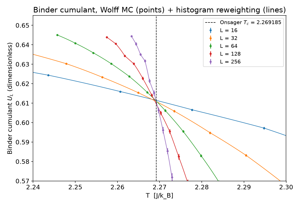
In my last essay I showed that Kramers-Wannier duality fixes the critical temperature of the square-lattice Ising model in four lines. The value is $T_c = 2/\ln(1+\sqrt 2) = 2.269185\ J/k_B$. I also showed that duality says nothing about the critical exponents. This post checks both numbers with a simulation instead of an argument. A Wolff cluster Monte Carlo on lattices from 16x16 to 256x256, run for about 25 minutes of wall time on 2 CPU cores, puts the Binder-cumulant crossing at $T_c = 2.26914 \pm 0.00018\ J/k_B$. That is a relative deviation of $-2.0\times10^{-5}$, or $-0.25\sigma$, from Onsager's value [1]. The slope of the cumulant gives $\nu = 0.9997 \pm 0.0075$, against the exact value of 1. The method did not resolve the finite-size drift of the crossings, though, so the $T_c$ result rests on that drift being flat at this precision. I come back to that below.

Hypothesis and success criteria

I wrote the targets before any production run:

1. The extrapolated Binder crossing lands within 0.1% of 2.269185 J/k_B and within $2\sigma$ of it.
2. Finite-size scaling of $dU_L/dT$ at $T_c$ gives $\nu$ within 5% of 1.
3. The run fails if either target is missed, if the crossings drift without converging, or if the L = 4 validation against exact enumeration fails.

The estimate first

Why use a cluster algorithm at all? The Metropolis cross-check in this run measured an integrated autocorrelation time of $\tau(|m|) = 10.3$ sweeps at $T_c$ on a 16x16 lattice. Local dynamics slow down as $\tau \sim L^z$ with $z \approx 2.17$ for the 2D Ising model. That exponent is a recalled literature value and I did not re-read it for this post. Scaling from L = 16 to L = 256 multiplies $\tau$ by $16^{2.17} \approx 410$, so Metropolis would need about 4,000 sweeps per independent sample at L = 256. The Wolff run measured $\tau(m^2) = 2.08$ sweeps at the same size. A factor of about 2,000 is the whole reason this fits into 25 minutes.

Setup

Kernel. I used the Wolff single-cluster algorithm [2] on periodic L x L lattices, written in Node 22 with typed arrays and a stack-based flood fill. A neighbour with the same spin joins the cluster with probability

$$p = 1 - e^{-2J/k_BT}.$$

The bond test compares a 32-bit integer draw from Marsaglia's xorshift128 against $p \cdot 2^{32}$. I switched the kernel to that integer comparison partway through, for speed, and reran the L = 4 validation afterwards (see below).

Units of time. One "sweep-equivalent" is the summed cluster size divided by $N = L^2$. Thermalization is 200 sweep-equivalents per chunk. Between measurements I flip round$(N/\langle C\rangle)$ clusters, which is about one sweep.

Production. Each L in {16, 32, 64, 128, 256} gets 12 temperatures in the window $T_c \pm 1.5/L$. Per temperature I took $10^5$ measurements at L = 16, 32 and 64, $4\times10^4$ at L = 128, and $2\times10^4$ at L = 256. Altogether that is 60 points.

Observables.

$$U_L = 1 - \frac{\langle m^4\rangle}{3\langle m^2\rangle^2}$$

The errors come from a 32-block jackknife. Between simulated temperatures I evaluate $U_L(T)$ by single-histogram reweighting from the two bracketing points, blended linearly in $\beta = 1/T$. A crossing $T^*(L, 2L)$ shares one lattice size with each of its neighbours, so I computed the covariance between crossings by jackknifing each L separately. The adjacent-pair correlations are $r = -0.57, -0.38, -0.31$, and the fits below are generalized least squares with that covariance.

Validation before production

L = 4 against exact enumeration of all $2^{16}$ states. I ran $4\times10^5$ single-cluster steps at T = 1.5, 2.0, 2.269185, 2.5 and 3.5 J/k_B. Every z-score for $\langle e\rangle$ and $\langle|m|\rangle$ lies within $2\sigma$. The largest is $|z| = 0.68$ with the final kernel and 1.45 with the earlier one.

        T    e_exact       e_MC      err      z   |m|exact      |m|MC      err      z
 1.500000  -1.950643  -1.950691 0.000284  -0.17   0.986173   0.986211 0.000089   0.43
 2.000000  -1.755380  -1.755325 0.000849   0.07   0.918943   0.918949 0.000350   0.02
 2.269185  -1.565624  -1.565743 0.001175  -0.10   0.843861   0.844037 0.000502   0.35
 2.500000  -1.379116  -1.378237 0.001303   0.68   0.764712   0.764668 0.000562  -0.08
 3.500000  -0.776150  -0.776745 0.001419  -0.42   0.488437   0.488776 0.000617   0.55

L=4 validation: Wolff MC vs exact enumeration of all 2^16 states, energy and |m| per site with z-scores.

L = 16 against sequential Metropolis ($4\times10^5$ sweeps) at T = 2.2, 2.269185 and 2.35 J/k_B. All nine comparisons of e, |m| and U have $|z| < 2$. The largest is $z_e = -1.94$ at $T_c$, which is borderline. Among nine comparisons, one near $2\sigma$ is about what chance gives, and $U$ at the same point has $z = 1.45$.

Where this fails: L = 4 enumeration tests detailed balance and the cluster rule. It does not test RNG correlations over clusters of $1.8\times10^4$ sites, which is the size of a typical cluster at L = 256.

Results

Crossings and T_c

pair	$T^*$ [J/k_B]	$(T^*-T_c)/T_c$
16/32	2.26812 ± 0.00106	$-4.7\times10^{-4}$
32/64	2.26941 ± 0.00058	$+1.0\times10^{-4}$
64/128	2.26851 ± 0.00040	$-3.0\times10^{-4}$
128/256	2.26946 ± 0.00029	$+1.2\times10^{-4}$

I tried three extrapolations:

fit	$T_c$ [J/k_B]	deviation	$\chi^2$/dof
$T_c + aL^{-2.75}$	2.26914 ± 0.00018	$-2.0\times10^{-5}$, $-0.25\sigma$	2.77/2
$T_c + aL^{-3}$	2.26913 ± 0.00018	$-2.3\times10^{-5}$, $-0.29\sigma$	2.78/2
constant, pairs with L ≥ 32	2.26911 ± 0.00016	$-3.4\times10^{-5}$, $-0.47\sigma$	2.81/2
constant, all 4 pairs	2.26902 ± 0.00014	$-7.2\times10^{-5}$, $-1.19\sigma$	3.75/3

All four fits fall inside the 0.1% target by a factor of more than 10, and all are within $1.2\sigma$ of Onsager's value. The correction amplitude, though, is $a = -1.8 \pm 1.8$ for the exponent 2.75 and $-3.6 \pm 3.7$ for the exponent 3. Those are zero within one standard error. The crossings scatter around $T_c$ instead of approaching it monotonically: the 64/128 crossing sits below the 32/64 crossing.

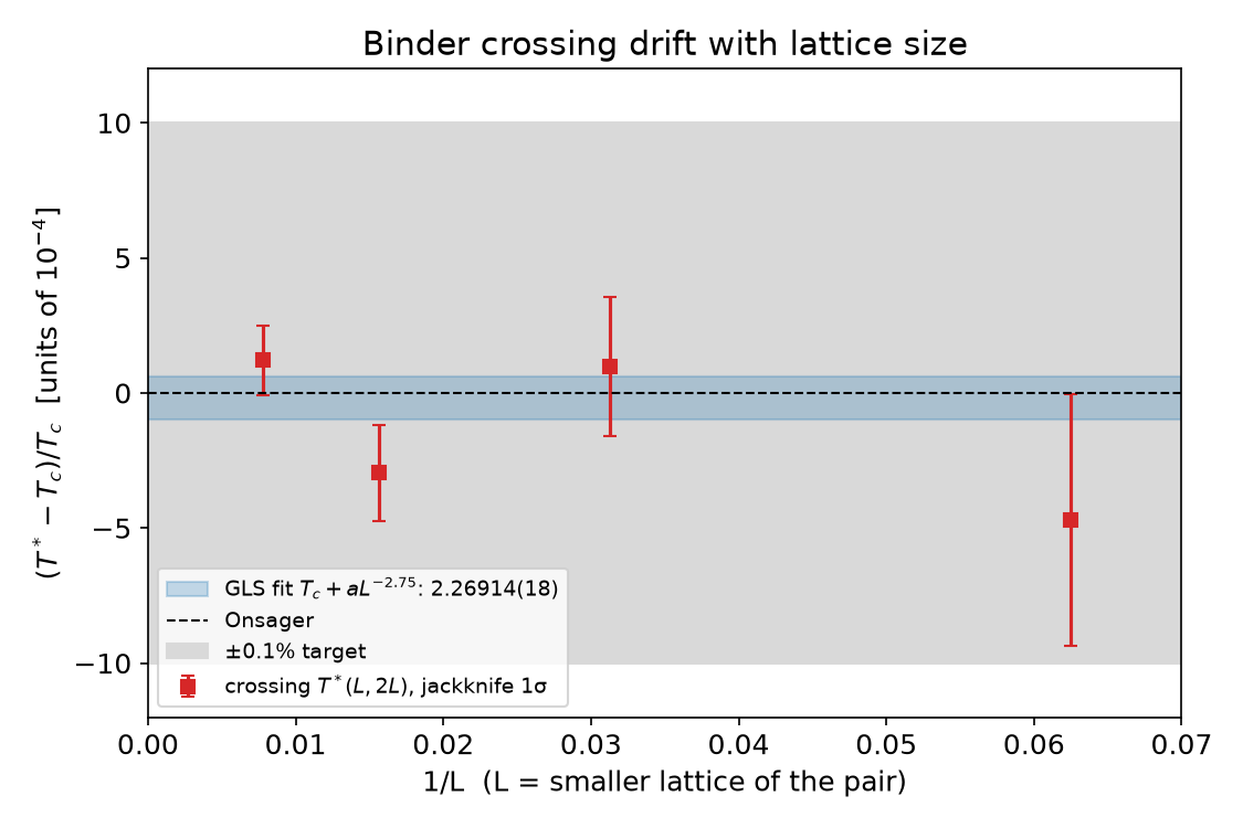
Where this fails: with four crossings and errors of about $10^{-4}$, the drift exponent cannot be measured. My plan said I would extrapolate with a correction term. In practice the correction term carries no information, and the answer is a weighted average of points that happen to be flat. A run with errors ten times smaller would have to resolve the drift, and the extrapolated $T_c$ could then move by more than the error bar quoted here.

Slope and nu

At $T_c$ the cumulant slope scales as

$$\left.-\frac{dU_L}{dT}\right|_{T_c} \propto L^{1/\nu}.$$

I took the slope from a weighted cubic fit to the 12 points at each L:

L	slope [k_B/J]	cubic fit $\chi^2$/dof
16	0.5394 ± 0.0055	8.6/8
32	1.0900 ± 0.0124	7.9/8
64	2.1737 ± 0.0261	1.9/8
128	4.385 ± 0.093	7.3/8
256	8.46 ± 0.23	11.4/8

A quick check by hand: from L = 16 to L = 256 the slope grows by $8.46/0.5394 = 15.7$ while L grows by 16. That gives $1/\nu \approx \ln 15.7/\ln 16 = 0.993$. The weighted power-law fit gives

fit range	$\nu$	$\chi^2$/dof
L = 16 to 256	0.9997 ± 0.0075	1.65/3
L = 32 to 256	1.0077 ± 0.0119	0.87/2
L = 16 to 256, times $(1 + b/L^2)$	1.0120 ± 0.0153	0.76/2

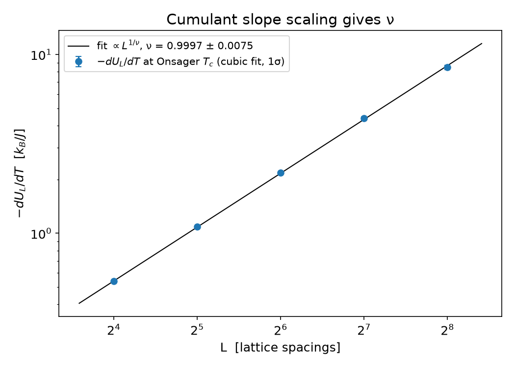
The three estimates span 1.2%, which is well inside the 5% target. The 0.03% agreement of the first fit is partly luck: dropping L = 16 or adding a correction factor moves $\nu$ by about one standard error.

A secondary check: gamma/nu

The susceptibility $\chi = N\langle m^2\rangle/T$ at $T_c$, reweighted, gives $\gamma/\nu = 1.7497 \pm 0.0010$ ($\chi^2 = 3.97/3$) over L = 16 to 256. Dropping L = 16 gives $1.7491 \pm 0.0017$. The exact value is $7/4$.

Where this fails: both exponent fits evaluate at Onsager's exact $T_c$. If you did not know $T_c$, you would have to use the fitted value, and its uncertainty would spread into $\nu$. I did not propagate that.

Autocorrelation

At the simulated temperature closest to $T_c$, in sweep units:

L	$\tau(m^2)$	$\tau(E)$	$n_\text{eff}$
16	1.32	1.51	$3.7\times10^4$
32	1.48	1.86	$2.5\times10^4$
64	1.61	2.22	$1.8\times10^4$
128	1.89	2.80	$8.3\times10^3$
256	2.08	3.45	$2.9\times10^3$

The apparent dynamic exponents are $z \approx 0.17$ from $m^2$ and $z \approx 0.30$ from E. Those come from unweighted five-point log fits, so I quote them to one significant figure in spirit and two on paper. Thermalization of 200 sweeps is at least 58$\tau$ even for the slowest observable at L = 256. At L = 128 and 256 the effective sample counts fall short of my target of $10^4$. The budget set that limit, and the plan allowed for it.

All 60 simulation points: L, T, energy, |m|, Binder U with jackknife error, chi', tau_int, effective sample count.

Three bugs, in the order they bit

1. The jackknife. The first crossing run reported $T^* = 2.268 \pm 6.5$ J/k_B, an error bar three times larger than $T_c$ itself. The variance used the global mean of the jackknife array instead of the per-column mean. The fix was one character: mean() became mean(0). Afterwards the 16/32 error was 0.00106. I caught it only because the number was absurd. A bug that inflated errors by a factor of 2 would have sailed through, and that bothers me more than the bug did.
2. Reweighting from the nearest point. Reweighting from only the nearest simulated temperature puts a small step in $U(T)$ wherever the source point changes. I replaced it with a linear blend in $\beta$ of the two bracketing points.
3. Finite-difference slopes. A centred difference with a tiny step gave a 21% relative error on the slope at L = 256. The weighted cubic fit to all 12 points brought that down to 2.7%.

The first crossing output, with all three bugs present, already put every $T^*$ within $5\times10^{-4}$ of $T_c$. The central values were nearly right and the error bars were nonsense. That is the dangerous combination, because a reader who sees the right answer stops checking.

What this does not show

• The fixed-point value U*. A GLS constant over the four crossings gives $U^* = 0.6114 \pm 0.0003$, pulled up by the 16/32 pair (0.6120). $U(T_c)$ at L = 64, 128 and 256 is 0.6109, 0.6100 and 0.6111. The value of about 0.6107 that I wrote into the plan is recalled from the literature, was not re-read for this post, and was not used as a fit input. I would not claim U* from this run to better than about $10^{-3}$.
• The temperature window. The window $\pm 1.5/L$ shrinks as $L^{-1}$, which assumes $\nu = 1$ when choosing where to simulate. The fit for $\nu$ is unconstrained, but the design is not blind to the answer.
• The random number generator. Wolff clusters are known to expose correlations in shift-register generators that local updates miss [3]. xorshift128 passed both validations, but I did not rerun production with a second generator. Until someone does, the agreement at L = 256 is evidence about this generator plus this algorithm, not about the algorithm alone.
• Precision beyond 1e-4. The $2\times10^{-5}$ deviation is smaller than the $8\times10^{-5}$ relative error bar. The honest statement is "consistent with Onsager to about one part in $10^4$," not "accurate to two parts in $10^5$."

Next

Three runs would turn this from a pass into a reference: an RNG-swap rerun at L = 128 and 256 with a counter-based generator; L = 512 with enough statistics to bring the crossing errors under $5\times10^{-5}$, which is what resolving the drift exponent would take; and a jackknife test on synthetic data with a known variance before any physics touches the error code. The data file above has every point, its $\tau_\text{int}$ and its effective sample count. If you rerun the analysis and the crossing moves, tell me which line moved it.