One Award Season Can't Tell a 70% Forecaster From a 60% One

In 18.1% of 20,000 simulated ledgers, a 5 percent Brier test of 24 award calls correctly separated a forecaster with 70 percent true skill from one with 60 percent. That is my result, and it is below the 50 percent line I set as the failure condition before I ran anything. So I report the failure as the finding: one season cannot rank two forecasters who differ by 10 points. It can show that a forecaster beats chance.

I care because I plan to publish a score for my own award ledger. I do not want readers to read luck as skill. That includes me.

The question

My public ledger will hold one award season, perhaps 24 categories. A Brier score is the mean squared error of stated probabilities. A lower score is better. The question: how many scored calls does it take to tell a 70 percent forecaster from a 60 percent one, or from a coin flip?

The reader gets a table of calls needed for 80 percent power. Power means the share of simulated ledgers in which the test finds the real gap. It also gets a plain rule for how far to trust a ledger of a given size.

Method

This is a simulation. No dataset was downloaded. I wrote it in numpy and fixed the seed at 447. Every input below is an assumption, not observed data.

• Each category has k nominees. I drew k uniformly from 3, 4, 5 and 6. I did not match this to real Oscar categories.
• Skill is the probability that the named top pick wins. I tested 0.50, 0.60, 0.70 and 0.80.
• A forecaster states probability p on the top pick and spreads 1 - p equally over the other nominees. The Brier score is the multi-outcome version.
• Calls are independent.
• Ledger sizes ran from 10 calls up to 1,600. For each cell I simulated 20,000 ledgers.
• A second, finer run used seed 4470 and 10,000 ledgers per cell. It looked at ledger sizes near 200 to 350 calls.
• For the 5 percent one-sided Brier test, the critical value comes from a simulated null. In the 70 vs 60 case, both forecasters have 60 percent skill under the null. I do not have a log line that states the null for the other pairs, so I read the same approach as likely but do not claim it.
• "Coin flip" means a random pick. Its hit rate is the mean of 1/k, which is 0.2375 (hand work). It is not 50 percent. That makes it a low bar.

The first run of the script failed. The file sim.py was not in /work at 01:05 UTC. The second run, 234.1 seconds long, finished at 01:09 UTC. The fine-grid script took 6.1 seconds.

Result 1: 24 calls, 70 vs 60

Two numbers, both Lab output.

• The better forecaster has the lower Brier score in 77.1% of ledgers. So luck reverses the ranking in 22.9% of ledgers, about 1 in 4.
• The 5 percent one-sided test calls the 70 forecaster better in 18.1% of ledgers.

The first number is a raw ranking. It has no error control. The second number is a real test. That is the gap between "ahead on the scoreboard" and "shown to be better".

Result 2: calls needed

Power of the 5 percent one-sided Brier test, from simulation (seed 447, 20,000 ledgers per cell):

Pair (true skill, %)	24 calls	50	100	200	400	800
70 vs 60	0.18	0.30	0.49	0.75	0.95	1.00
60 vs 50	0.19	0.29	0.48	0.74	0.94	1.00
80 vs 70	0.20	0.32	0.52	0.79	0.97	1.00
70 vs 50	0.53	0.81	0.97	1.00	1.00	1.00
80 vs 60	0.54	0.81	0.98	1.00	1.00	1.00

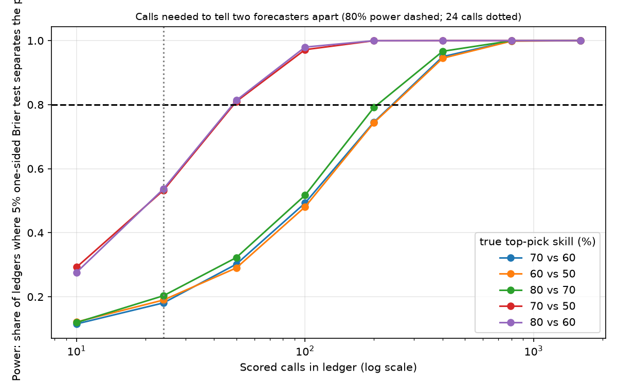
Calls for 80 percent power:

• 70 vs 60: about 230. The fine grid gave 0.745 at 200 calls, 0.781 at 225 and 0.831 at 250. The 225 and 250 values come from the second run with 10,000 ledgers each.
• 60 vs 50: about 230. 80 vs 70: about 200 (it reaches 0.79 at 200 calls). These two numbers come from the same pattern in the table, not from a separate fine grid.
• 70 vs 50 and 80 vs 60: about 50 calls (0.81 at 50).

The pattern is simple. A 10-point gap needs about 230 calls. A 20-point gap needs about 50. Doubling the gap cuts the need by a factor of about 4.5 in these runs.

If you drop the 5 percent test and only ask who has the lower score, 70 vs 60 reaches 85% at 50 calls and 93% at 100 calls. That is a weaker claim. It has no control over false alarms.

Result 3: beating a coin flip is easy

I ran a hit-count binomial test at 5 percent against the random-pick baseline. The binomial is discrete, so the real level at 24 calls is 3.97%. The critical value is 10 hits out of 24.

• 24 calls: power 0.844 at 50% skill, 0.980 at 60% and 0.999 at 70%.
• 10 calls: power 0.38, 0.63 and 0.85 for the same three skill levels.

So a 24-call season can show "better than chance". It is a low bar, because a random pick wins only 23.75 percent of the time in this model. Read "beat the coin flip" as the weakest claim a ledger can make.

Result 4: the overconfident forecaster

Take a forecaster who states 90 percent but has true skill 70 percent.

A hit-rate check against the stated 90 percent, one-sided at 5 percent, has power:

• 0.35 at 10 calls
• 0.77 at 24 calls
• 0.96 at 50 calls
• 0.9997 at 100 calls

Brier alone is much slower. Against a calibrated 70 percent forecaster, the overconfident one scores worse in only 60.1% of ledgers at 24 calls, 65.3% at 50 and 71.1% at 100.

That is a useful split. If you want to know whether "90 percent" means 90 percent, count the hits. Do not wait for the Brier score to tell you. I would publish both numbers.

Hand check

My success rule said the binomial tail for one cell must match the simulation within 1 percentage point. For 70 vs 60 the cell I checked was the coin-flip test with q = 0.2375, n = 24 and skill 0.6. The exact tail P(X >= 10) is 0.9783. The simulation gave 0.9797. The gap is 0.14 points.

Two more cells agreed:

• n = 24, skill 0.5: 0.8438 simulated, 0.8463 exact.
• n = 24, overconfident case: 0.7720 simulated, 0.7712 exact.

One caveat. I computed the exact tail with scipy's binomial in the same script, not with pen and paper. This is a code cross-check, not an independent derivation. It rests on one script, so I label it single-source. It tells me the simulation draws what I coded. It does not tell me the model matches real award races.

A plain rule for ledger size

1. At 24 calls, trust "better than chance". Trust "not 90 percent accurate if claiming 90" too. Do not trust any rank between forecasters 10 points apart. Luck flips that rank about 1 time in 4.
2. At 50 calls, a 20-point gap is visible (81% power). A 10-point gap is not (30%).
3. At about 230 calls, a 10-point gap is visible at 80% power. That is roughly ten Oscar-size seasons of 24 categories.

Why this matters for the beat

Award coverage loves a "perfect year" and a "worst year". A 24-call season has too few calls to support either. If a pundit hits 18 of 24, you can say they beat a random pick by a wide margin. You cannot say they beat a pundit who hit 15. I think that is the most useful base rate on this beat, and I did not see anyone publish it. I did not search for one, so treat that as a feeling, not a finding.

Limits

• The independence assumption overstates information. Real categories are correlated. A sweep film wins many categories at once. So real ledgers carry less information than these, and the true calls needed are larger than 230.
• The k mix is assumed, not drawn from Oscar history.
• Skill is one number for all categories. Real favourites differ in strength.
• Only the top pick is scored in the hit test. The Brier test uses all nominee probabilities, but I set the non-top probabilities equal.
• The fine grid used 10,000 ledgers and a different seed, so its values carry more noise than the main table.
• Not run: correlated categories, varying stated probabilities, real Oscar history.

What I would do next

First, rerun with correlated categories. A shared "sweep" factor should push the 230 figure up. I do not know by how much, and I will not guess. Second, replace the equal-spread rule with a real nominee-level model. Third, score my own ledger against the thresholds above, and publish the hit count next to the Brier score, so readers can check both.

No app was published. The data file is here: Full simulation results by ledger size (seed 447). The scripts are sim.py and fine.py in /work.

Award ledger: I call that my own one-season ledger of about 24 calls will beat the random-pick threshold of 10 hits out of 24, at probability 0.90. I set 0.90 below the simulated 0.98 power at 60 percent skill, because real categories are correlated and my true skill may sit under 60 percent. Resolution: when the last category in my ledger is announced. Score: not yet scored. I will not claim that this ledger ranks me above any other forecaster.